Recent Improvements and Fixes
This page lists recent improvements and fixes to the particle–gas coupling: interpolating the gas to the particles, projecting the particles back onto the mesh, the drag and heat closures, particle collisions with each other and with walls, memory, and conservation across MPI ranks and periodic boundaries. For each: what was wrong, how it was fixed, and how the fix was checked.
All changes are covered by the regression suite in Regression Tests: 67 cases, compared against stored goldens and checked against physics on 1, 2 and 4 ranks, and one unit test.
Summary
| Area | Problem | Fix | Commit |
|---|---|---|---|
| Interpolation | Inverse distance (1/d³) had errors of up to ±18% of the change in density across one cell, even in a linear field, and was discontinuous at cell faces. A particle sheet hit by a planar shock rippled with the cell size (57 µm standard deviation after 250 µs) | Weighted linear least squares, exact for linear fields; the sheet stays flat (0.07 µm) | 89f9661, 6d00ca4 |
| Projection | The kernel used one length for every direction, so the spread on stretched cells was wrong | Each direction is scaled by its own cell length | 414ce7f |
| Projection | Cells just outside the bin domain were dropped, so cloud-edge particles reached 8 cells instead of 27; φ was ~8% too high at the edge | Map those cells to particle bins | affad85 |
| Closures | Forces and heat transfer were skipped below 1 mm/s slip, and the old value was kept | Evaluate at any slip; skip only the quasi-steady drag at zero slip | f0ae123 |
| Quasi-steady drag | Gidaspow's C_D was capped below Re = 0.1 (100% error); Osnes had a spurious Knudsen reduction (25% error) | Correlations match the published ones; QSFORCE renumbered | 94607fd |
| Heat transfer | Gunn's and Sun's Nusselt correlations were evaluated with the particle Reynolds number Re_p instead of the mean slip Reynolds number Re_m = ε_f Re_p they were fitted with: Nu up to 35% too high (Sun) and 62% (Gunn) at ε_s = 0.5 | Both use Re_m; Sun's Nu is within 7.9% of its PR-DNS data on average (20.9% before) | 3c677d9 |
| Heat transfer | Sun's correlation, fitted for ε_s = 0.1–0.5, was extrapolated below 0.1: as ε_s → 0 the per-particle Nu went to π/2 instead of 2, 33–41% below a single sphere at Re_m = 1–100 | Below ε_s = 0.1, Sun's value at 0.1 is blended into Ranz–Marshall | 955ba8e |
| MPI | Gas state in virtual cells was stale at rank borders with particles, setting the gas around a quiescent cloud moving (1e-4 m/s) on 2+ ranks; total gas energy differed from 1 rank by 5e-8 | Convert and re-exchange after φ is known; exchange φ every stage | e3ed370 |
| Conservation | Fluxes on periodic and symmetry patches were not conservative | Exchange and transform gradients in virtual cells | 11dc640 |
| Robustness | A single particle gave a filter width of 0 | Filter width from cell–box overlap | 48f64b7 |
| Build | Required SPEC=1 |
Builds without it; stops if species are requested | aa3c0b6 |
| Random numbers | QS fluctuations drew from one generator per rank, every rank seeded with 1: the same noise on every rank, and results that changed with the number of ranks | Each particle has its own stream (splitmix32), seeded with its line in points.dat and carried with the particle; 1 and 2 ranks now give identical results |
(section "Random numbers for the stochastic models") |
| Collisions | The contact stiffness used particle i's own mass, so an unequal pair felt unequal forces: an 8:1 pair at 20 m/s ended with its total momentum reversed | Stiffness from the pair's effective mass (soft-sphere model) | 3afd23a, 78eb711 |
| Particle walls | Walls existed only through filein.vtk; a particle over the edge between two wall triangles was pushed by both (e = 0.60 instead of 0.70); a fast particle went through the wall and the run crashed |
Walls from the fluid wall patches (PARTWALL 1), contacts computed like pair contacts, a fluid side that pushes back; filein.vtk removed |
2ff0cd8 |
| Ghost particles | Overflowing the ghost arrays wrote past their end | Guards stop the run; ghost arrays 30% smaller | f7a3980, 0bb2e4b |
| Neighbour search | Dense subbin tables: ~28 GB requested for 50,000 particles in one 2 cm bin | Compact lists: ~1.2 MB for the same bin (about 24,000 times less), byte-identical results | 82d4ca4 |
| Clean-up | ppiclF's own unit tests no longer matched the code; the burn-rate model and the PICLDEBUG output were unused |
Removed; the regression suite replaces the unit tests. Input files that still ask for REACTIVE or a negative STATIONARY stop with a message |
3c41db2 |
| Memory | ppiclF reserved fixed arrays for 80,000 particles, 640,000 ghosts and 120,000 cells per rank, plus 50 steps of viscous-unsteady history even when it was off: 1.34 GB for a run with one particle. A run with more particles on a rank stopped and needed a recompile | Arrays sized from the run and grown when needed; the history is allocated only with VISCOUSUNSTEADY (VUSTEPS steps). 265 MB for the same run; no particle, ghost, cell or wall limits |
c1ac692, 0d4d86c, e227f99 |
| Particle output | Every file held all 72 particle fields, named y01…, rpro01…, tag01… (300 bytes per particle) |
A list of named fields: velocity, volume fraction, diameter and ID by default (44 bytes per particle); more groups with PARTICLE_WRT, GAS_WRT, GRADGAS_WRT, MODEL_WRT. Restarts read the particle dump in restart_data/ (Input File) |
(this section) |
| Interpolation speed | 60% of a particle stage went to finding the cells around each particle | Marker per cell, an early exit and contiguous reads: that search is 45% faster, the whole run 14–20% faster, results bit-identical | (section "Where a particle stage spends its time") |
| Ghost particles | A ghost carried all 59 particle properties; the neighbour search reads 6 | A ghost carries those 6 (16 doubles instead of 69), byte-identical results | a7f5748 |
| Field sizes | The number of fields per particle and per cell (state, properties, interpolated, projected) was fixed at compile time; Rocflu's number of interpolated fields had to match it by hand; every run interpolated 29 gas fields and projected 31 | Set at start-up by ppiclf_user_Layout from the physics that is on: 7 interpolated fields for drag only; ppiclF stops if a needed field is not given; byte-identical flow files |
074d58d, (section "Field sizes set at run time") |
| Input | Mistakes in the input were found at run time, after the job started, or never: a typo or misplaced key was silently ignored, QSFLUCT ran without a drag, unused keys (FILTERWIDTH, angular periodicity, REACTIVE) had to be given; the particle material came from # MATERIAL by name; the build without particles did not compile |
Case validator (./rocflu.sh validate, run first by rocflu.sh run and the suite) checks keys, values, model combinations, points.dat and the particles' position before anything is built (Input File); VELOCITYMODEL replaces STATIONARY; DENSITY, SPECIFICHEAT in # PICL; points.dat is x y z vx vy vz dp; --no-picl builds and runs |
2b0c7a7, 59da501, 488e5df, b12cb48, 88542ac, 9d8be80, 4add494 |
| Particle bins | A particle bed stretched along one direction stopped the run with "Error in Createbins": the bin count split the bins with a wrong formula and went on with too many bins when its search failed (12% of bin boxes in a scan) | Bins added one at a time to the direction with the longest bins; valid for every box. Unit test in the suite | 0688f68, 0887252 |
| 2D | ppiclF stopped unless it was in 3D, so a 2D case had to run as a thin 3D one | DIMENS 2 sets ppiclf_ndim 2: bins, ghosts, interpolation, projection, neighbour search and walls work in the plane; about 11 times faster on the wedge |
e687f98 |
| Time step | Virtual faces counted in the CFL sum, so a thin 2D mesh took more steps (2227 at Δz = 0.1 mm against 403 at 10 mm) | Left out: 385 steps at every thickness, and stricter case checks | 6016d2a |
| Particle gradients | The particle forces used the gas solver's WENO-smoothed gradients: at a shock a particle got 58% of the pressure-gradient impulse | A separate least-squares fit with the resolvable second derivatives, without WENO or limiter: the impulse is exact to 0.1%, and no false wall-normal gradient (30% with a linear fit) | 2c93e55 |
Regression Tests
Every fix on this branch is guarded by the suite in Regression Tests. It runs small cases of the full code (grid, pre-processing, Rocflu and ppiclF) and judges each one in two ways: against a stored golden, which catches any change, and against physics checks (conservation, exact interpolation of a linear field, restitution, decomposition independence), which say whether the result is right. The cases are:
- Shock tube (15 cases): a Mach 1.27 shock over 1, 2 or 4 particles, one- and two-way, with each force model switched on in turn (added mass, pressure gradient, viscous unsteady, heat transfer, quasi-steady fluctuations, Parmar and Gidaspow drag).
- Box (25 cases): an 8 mm cube, periodic or closed. Momentum and energy exchange, a quiescent cloud, heat exchange at rest, interpolation of a linear field, the projection on elongated cells, collisions through ghosts and periodic faces, binary collisions, and particle–wall collisions.
- Gas only (6 cases): a pressure jump in a closed, a periodic and a symmetry box, testing the flow solver's own conservation.
- 2D (21 cases): the coupling, interpolation, projection, collisions, walls and gas
conservation with
DIMENS 2(see 2D Runs). - Unit (1 test): ppiclF's bin count, without MPI (see Particle Bins).
Most cases run on 1, 2 and 4 ranks and must give the same particles on each. To run
them, from tests/:
module purge; module load gcc/14.2.0 openmpi/5.0.7
./run_tests.py run                     # all 67 cases and the unit test
./run_tests.py run -o box/walls        # a subset
Regression Tests lists every case and check, and explains how to run on a login node or through Slurm, read a failure and regenerate goldens after an intended change.
Interpolation: Weighted Linear Least Squares
A tracer moves across cells in a gas whose density varies linearly in x. Each cell centre holds the exact value, so a correct interpolation returns the straight line.
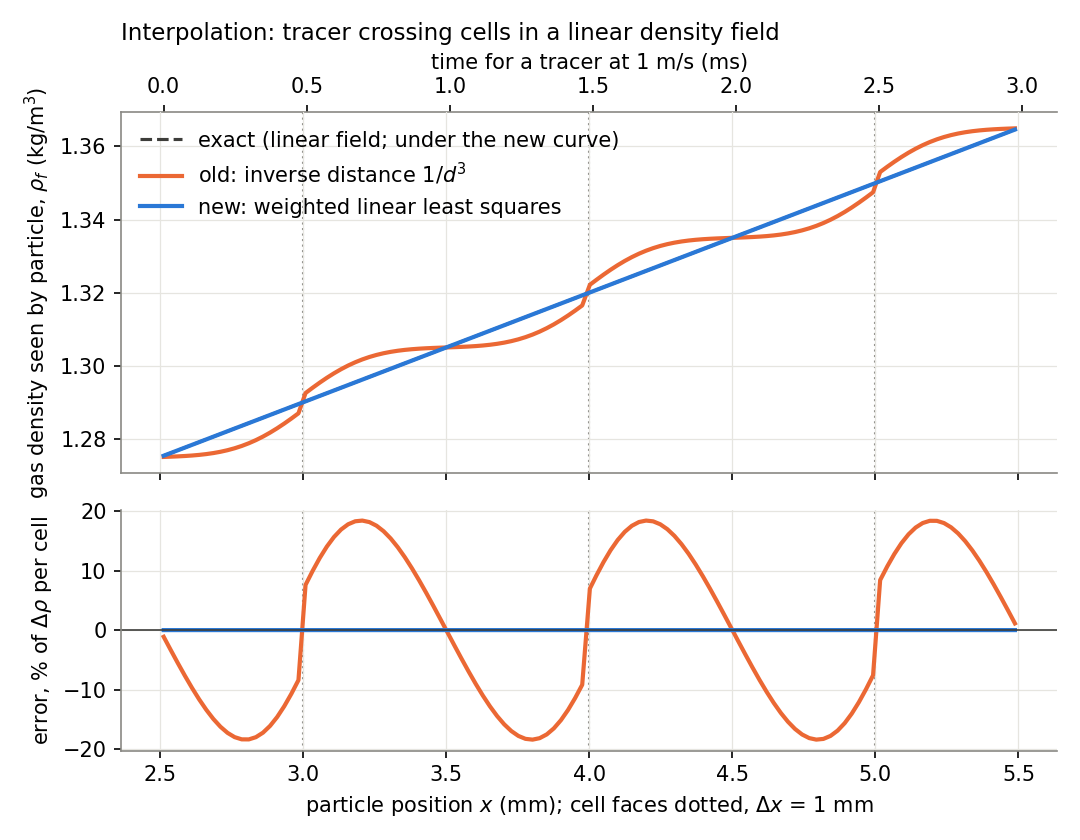
The old 1/d³ weighting pulled the value towards the nearest cell centre. The result was a staircase with errors of up to ±18% of the density change across one cell, and it jumped at every face. Weighted linear least squares (radius 1.8h) reproduces linear fields to round-off, and its value is continuous as the particle crosses a face. Each cell also now enters each bin's stencil only once; before, a two-bin periodic case counted some cells twice.
Choosing the Interpolation Method
Rocflu stores each field as one value per cell, at the cell centroid. ppiclF has to turn those values into the value at a particle. Four common ways to do it:
- Inverse distance (Shepard, 1968; the old ppiclF method): a weighted mean of the nearby cell values, weight 1/d³. ppiclF used the cells within 1.5 cell lengths.
- Trilinear: the 8 cell centres around the particle form a box; the value is the product of linear interpolations in x, y and z.
- Barycentric: the cell centres are split into tetrahedra; the value is the linear function through the 4 corners of the tetrahedron that contains the particle. Finding that tetrahedron is a point-location search on the dual mesh, as for particles on unstructured grids (Haselbacher, Najjar and Ferry, 2007).
- Weighted linear least squares (moving least squares, Lancaster and Salkauskas, 1981;
the current method,
ppiclf_solve_InterpLS): fit a + b·(x − x_p) to the cells within R = 1.8 cell lengths in each direction, each cell weighted by Π_l (1 − (Δx_l/R)²)⁶, and take a, clamped to the range of the stencil's values.
| Inverse distance | Trilinear | Barycentric | Least squares | |
|---|---|---|---|---|
| Cells used | about 27 | 8 | 4 | up to 64 |
| Exact for a linear field | no | yes | yes | yes |
| Continuous as the particle moves | no | yes | yes | yes, and smooth |
| Passes through the cell values | yes | yes | yes | no (a local fit) |
| Needs to know the mesh | no | the box of 8 centres (structured, hexahedral) | tetrahedra of the centres, and a search for the one containing the particle | no: only the nearby centroids |
| Irregular or unstructured cells | yes | no | yes | yes |
| Next to a wall | no box: needs ghost values or one-sided formulas | outside the tetrahedra: needs the same | fewer cells, still a linear fit |
ppiclF gets no mesh connectivity from Rocflu: each cell arrives as its centroid, its
extent in x, y and z and its volume (ppiclf_comm_InitOverlapGrid). A cloud of nearby
centroids is what its stencil search already returns, and that is all least squares
needs. Trilinear needs to know which 8 centres form the box around the particle;
barycentric needs a tetrahedral mesh of the centres, kept consistent across bins and
ranks. Both would need ghost values or special formulas near walls, where the particle
lies outside the box or the tetrahedra of the centres.
How the four compare on the same cell-centred data (a stand-alone model, not ppiclF; the least-squares part uses ppiclF's weights, radius and clamp):
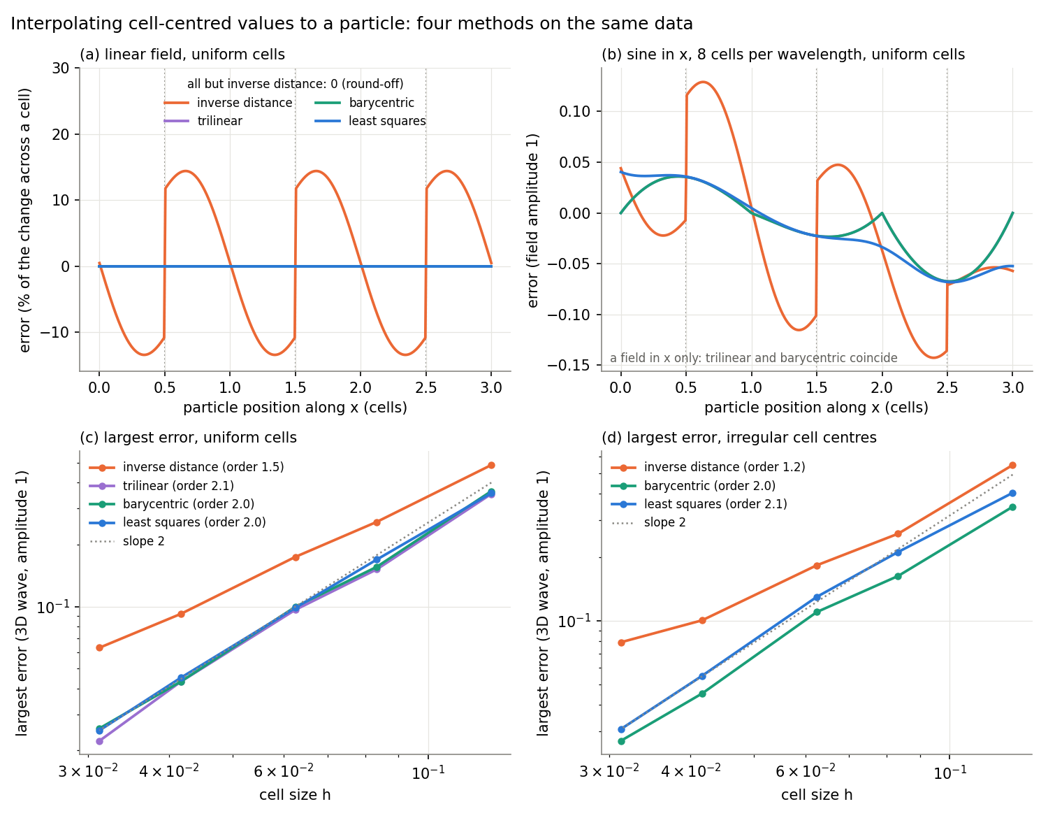
- (a) Linear field. Inverse distance is off by up to 14% of the change across one cell and jumps at every face. The other three are exact.
- (b) A sine along x, 8 cells per wavelength. Trilinear and barycentric pass through the cell values (zero error at the centres, a kink at each one); least squares does not pass through them, but its error is about the same size (largest 0.068 against 0.067) and it varies smoothly. Inverse distance has twice the error and jumps of 0.08 at the faces.
- (c) Uniform cells, a 3D wave. Trilinear, barycentric and least squares are second order, with errors within 20% of each other (0.022–0.026 at 32 cells across). Inverse distance converges more slowly and is 2.5 times worse at the finest mesh.
- (d) Irregular cell centres (each moved by up to ±0.2 cell lengths, as the centroids of an unstructured mesh). Trilinear does not apply. Barycentric and least squares stay second order; least squares' error is 15–30% larger than barycentric's. Inverse distance falls to about first order.
So least squares is as accurate as trilinear and barycentric (same order, similar errors), works on any cell layout, and needs nothing from the mesh but the centroids. What it costs: a wider stencil (up to 64 cells), one small (at most 4×4) solve per particle, shared by all fields, and a fit that does not pass through the cell values, so it can overshoot them and is clamped. On a regular hexahedral mesh, trilinear is cheaper and equally accurate, and is also exact for bilinear terms such as xy. Higher order schemes (cubic splines, Taylor series) need structured grids and more cells (Yeung and Pope, 1988).
References:
- D. Shepard, "A two-dimensional interpolation function for irregularly-spaced data," Proc. 23rd ACM National Conference, 517–524 (1968), doi:10.1145/800186.810616.
- P. Lancaster and K. Salkauskas, "Surfaces generated by moving least squares methods," Mathematics of Computation 37, 141–158 (1981), AMS.
- P. K. Yeung and S. B. Pope, "An algorithm for tracking fluid particles in numerical simulations of homogeneous turbulence," J. Comput. Phys. 79, 373–416 (1988).
- A. Haselbacher, F. M. Najjar and J. P. Ferry, "An efficient and robust particle-localization algorithm for unstructured grids," J. Comput. Phys. 225, 2198–2213 (2007).
Interpolation in Shock-Driven Flows
Same instant, different places in the cells. Stationary tracers sit at four fixed x positions in a planar shock (Ms 1.27, 1 mm cells): one behind the shock and three inside it. At each x they are stepped every 50 µm in y across four cells. The gas does not vary in y, so all tracers at one x must read the same value.
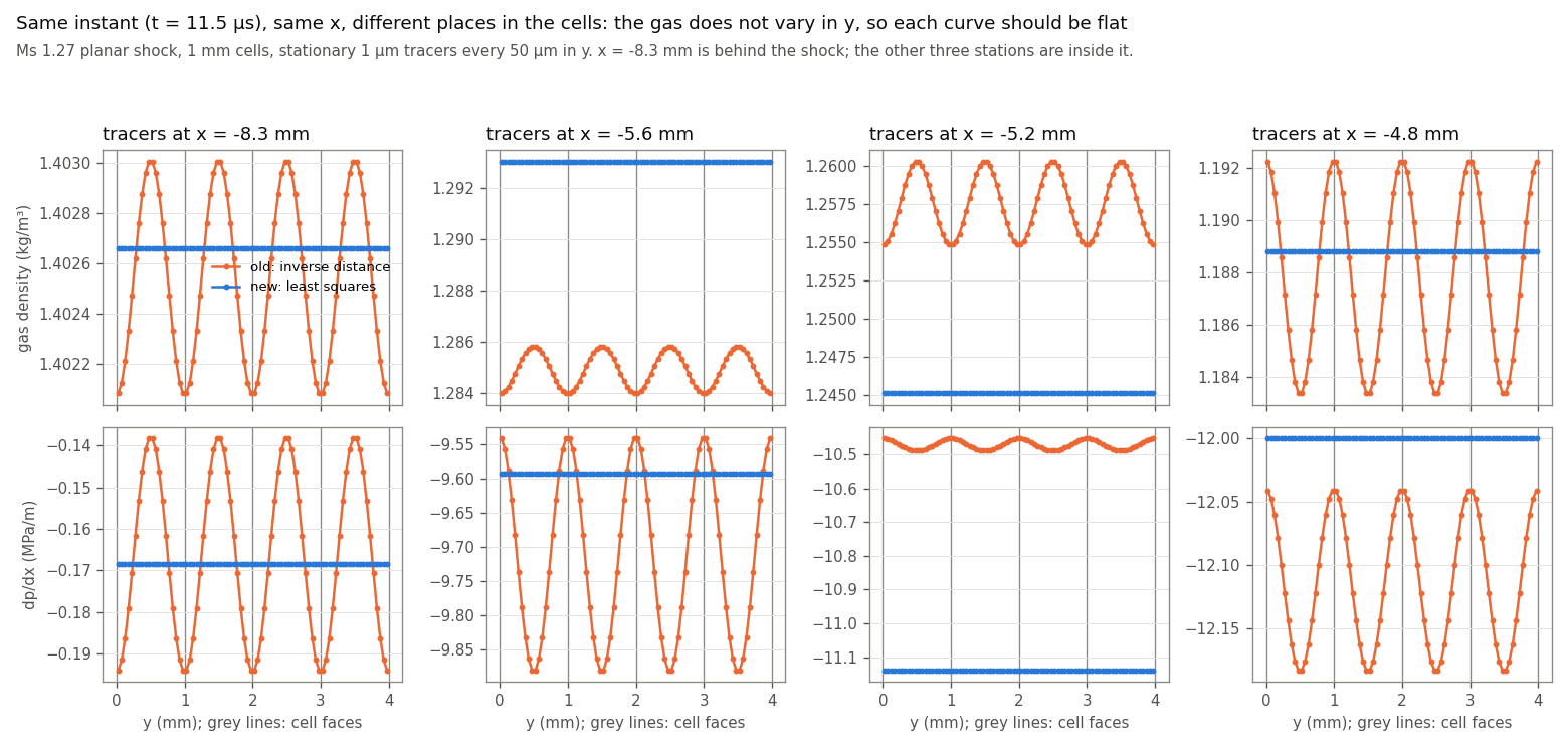
The old interpolation gives a wave with exactly the cell period: up to 0.7% peak to peak in density and up to 33% in dp/dx. The new one is flat. This is the y-direction counterpart of the interpolation figure above, where a particle moved along x.
The cause is the inverse-distance weighting. It weights each cell by its 3D distance from the particle, so a particle near a y face, roughly equidistant from several cell centres, gives more weight to the cells upstream and downstream of it in x than a particle at the cell centre does. Wherever the gas varies in x, particles at different places in their cells therefore read different values. Least squares fits a linear variation exactly, wherever the particle sits.
A particle sheet ripples with the old interpolation. A flat sheet of identical particles hit by a planar shock should stay flat: in a point-particle model nothing sets one particle apart from another. In the LLNL sheet case (8,281 particles, dp = 150 µm, Ms 1.27, cells 0.25 × 0.517 × 0.517 mm, run with the old code) it did not. The sheet sits in one layer of cells, so the gas density, volume fraction and pressure gradient change a lot from one x-cell to the next right at the sheet. Through the effect above, the particles read gas density differing by up to 4%, volume fraction by up to 38% and dp/dx by up to 40%, all from cells that are uniform in y and z to 0.4%. Particles on cell faces lagged and particles in cell centres led, so the sheet rippled with the cell size as wavelength; the standard deviation of the particles' x positions reached 193 µm (1.3 diameters) by 0.5 ms.
A periodic slice of that case (4 × 4 cells across, 13 × 13 particles at 13 different places in their cells, the same forces, two-way coupled) reproduces it:
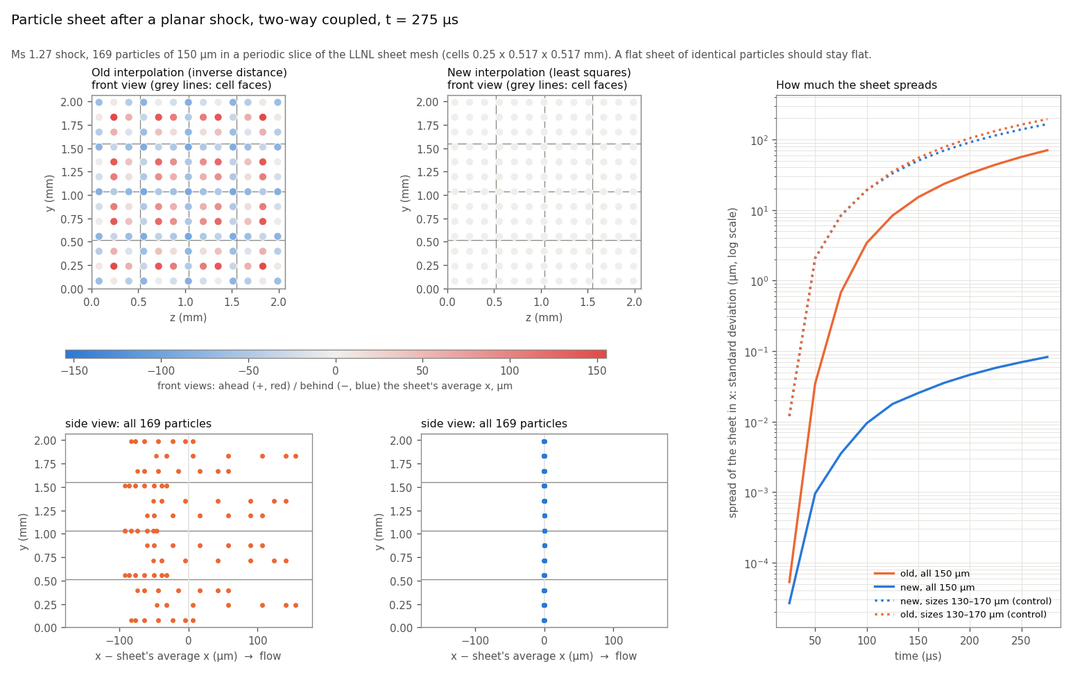
- Front views (top): the sheet seen face-on (z horizontal, y vertical), each particle coloured by how far it is ahead (red) or behind (blue) the sheet's average position. Old: a pattern tied to the cells. New: uniform.
- Side views (bottom): x horizontal (flow to the right), y vertical. Old: one bulge per cell. New: a straight line.
- Right: the spread of the sheet in x (standard deviation) over time, on a log axis.
| Spread of the sheet in x (standard deviation) | 100 µs | 150 µs | 200 µs | 250 µs |
|---|---|---|---|---|
Old, one-way (FEEDBACK 0) |
2.2 µm | 11.2 µm | 24.9 µm | 42.8 µm |
Old, two-way (FEEDBACK 1) |
3.4 µm | 15.2 µm | 33.1 µm | 56.6 µm |
| New, one-way | 0.09 µm | 0.24 µm | 0.48 µm | 0.78 µm |
| New, two-way | 0.01 µm | 0.03 µm | 0.05 µm | 0.07 µm |
The ripple appears with one-way coupling too, where the particles do not change the gas, so it comes from the interpolation and not from the feedback.
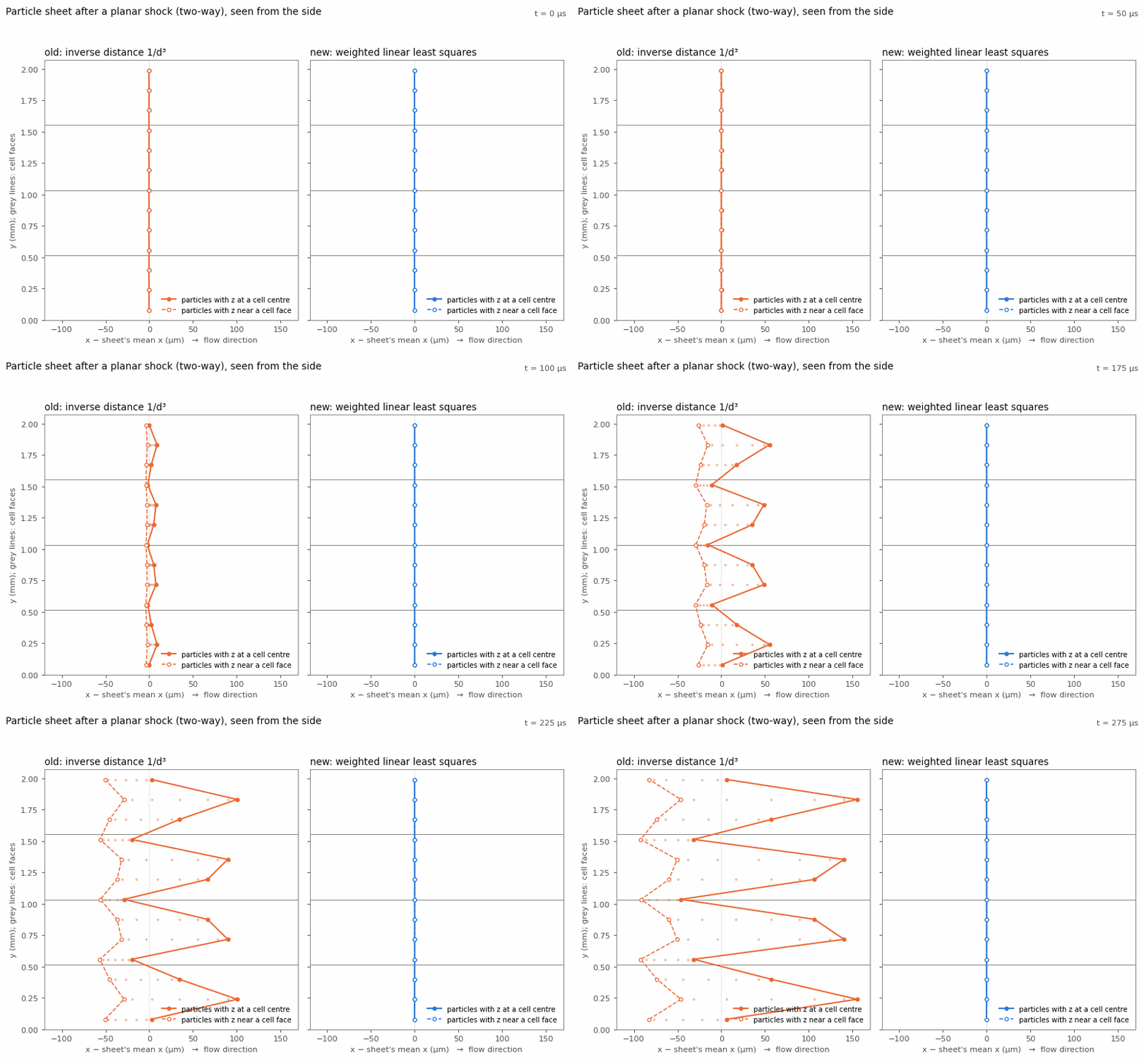
In the animation the solid line joins the particles whose z is at a cell centre, the dashed line those whose z is near a cell face.
Control: a sheet that must spread. With diameters from 130 to 170 µm the particles feel different drag (acceleration roughly as 1/dp), and the new interpolation spreads the sheet as it should: the 130 µm particles end 426 µm ahead of the 170 µm ones at 250 µs. The old run spreads a little more, because its cell-dependent push adds to the real one. The two are independent, so they add roughly as √(a² + b²):
| t | New, mixed sizes | Old artefact alone (identical particles) | √(sum of squares) | Old, mixed sizes |
|---|---|---|---|---|
| 150 µs | 50 µm | 15 µm | 52 µm | 55 µm |
| 200 µs | 91 µm | 33 µm | 97 µm | 104 µm |
| 250 µs | 139 µm | 57 µm | 150 µm | 163 µm |
So the new interpolation removes only the part of the spreading that depends on where particles sit in their cells. Where the real spreading is large, the old artefact was a 10–20% error on top of it; where it is small, as for identical particles, the artefact was all of it.
Shock profiles. The gas seen by a line of stationary 1 µm tracers across a planar shock (one-way), at two Mach numbers and two cell sizes:
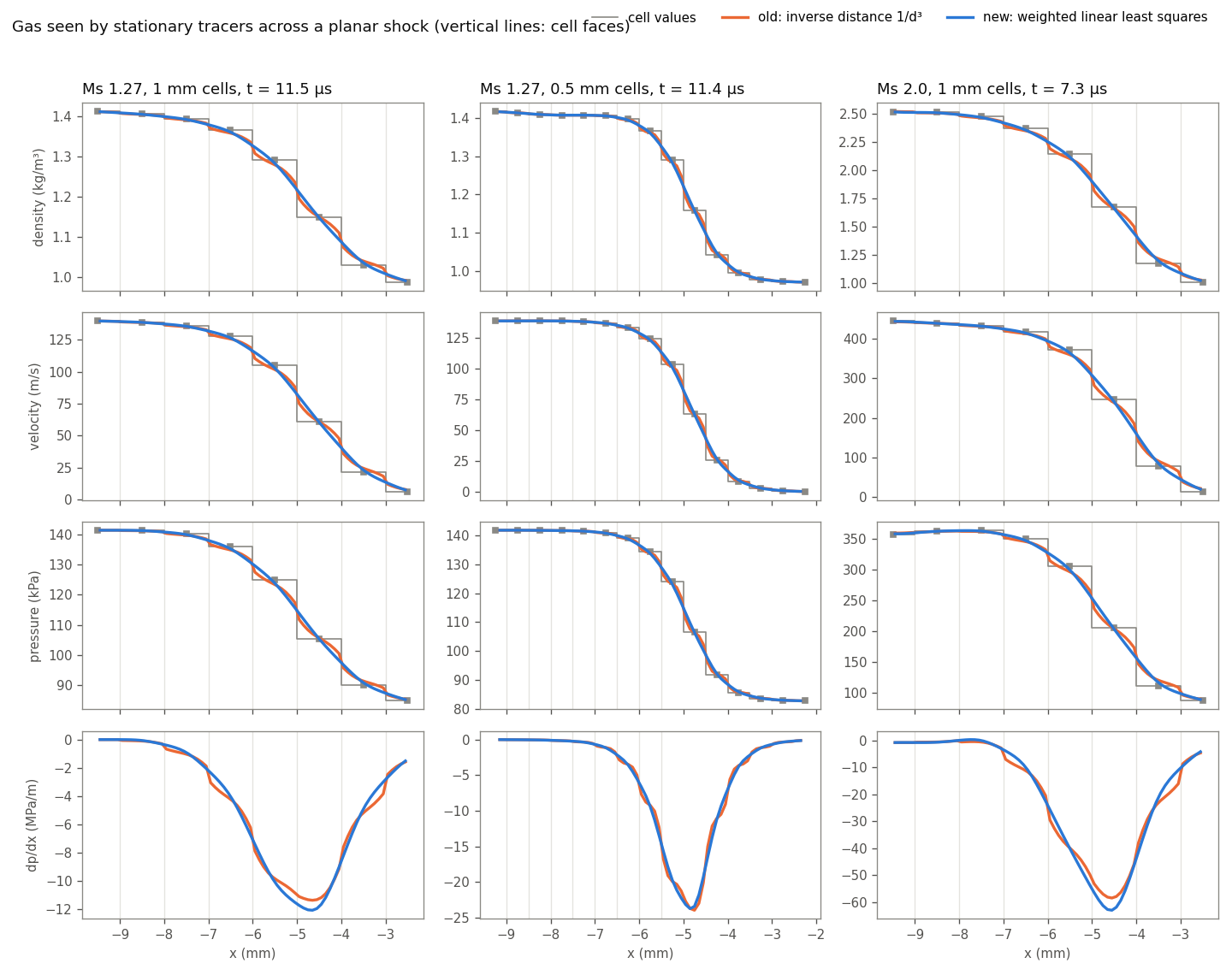
| Shock width 10–90% (density / pressure) | Cell values | Old | New |
|---|---|---|---|
| Ms 1.27, 1 mm cells | 3.69 / 3.29 mm | 3.86 / 3.67 mm | 3.49 / 3.31 mm |
| Ms 1.27, 0.5 mm cells | 1.94 / 1.91 mm | 1.99 / 1.99 mm | 1.92 / 1.92 mm |
| Ms 2.0, 1 mm cells | 3.77 / 2.86 mm | 3.68 / 3.00 mm | 3.32 / 2.81 mm |
"Cell values" is the straight line between neighbouring cell centres. Rocflu spreads the shock over 3–4 cells, and that width halves with the cell size. Least squares follows the cell profile and does not widen it (its support radius is 1.8 cells, but the fit is linear). Neither method overshoots the range of the cell values. The old method has kinks at every cell face, clearest in dp/dx (bottom row), so a particle crossing a face felt a sudden change in its pressure-gradient force. Both methods converge to the same profile when the cells are halved.
Where a Particle Stage Spends Its Time, and a Faster Stencil Search
Measured Breakdown
Case: periodic 8 mm box, 32³ cells, 50,653 particles (a 37³ lattice, dp = 100 µm), gas at 50 m/s, two-way coupling, 4 ranks on one node, 75 steps (210 RK stages timed). Each phase was timed with a barrier before and after it (temporary timers, not committed), so a phase is not charged for waiting on a slower rank. Times are for the whole run, per rank.
| Part of the particle stage (QS drag only) | Time | Share | Scales with the number of fields |
|---|---|---|---|
Stencil search: the cells around each particle (SBParticleToCellMap) |
28.9 s | 60% | no |
Least-squares fit: weights and the 4×4 solve (InterpLS) |
2.4 s | 5% | no |
Evaluating the 29 interpolated fields (InterpLS) |
3.9 s | 8% | yes |
| Copying the fields and sending them to the bins | 1.3 s | 3% | yes |
| Projection (31 fields) | 4.7 s | 10% | partly |
| Rocflu computing the gas fields before ppiclF | 3.8 s | 8% | mostly |
| Moving particles between bins, ghosts, forces | 2.8 s | 6% | no |
| Particle stage total (of a 60 s run) | 47.7 s |
Turning off bounds checking (-fcheck=all in ppiclF's flags, set in CMakeLists.txt) changes the run
time by about 2%, so it is not worth losing. perf on one rank put 52% of all samples in
SBParticleToCellMap.
So most of the time goes into finding the cells around each particle, not into the number of fields: sizing the fields at run time saves about 15% of a QS-only run; the stencil search was the larger target.
A Faster Stencil Search
For every particle, SBParticleToCellMap scans the cells of the 27 subbins around it (about 150
cells; subbins are 1.8 cell lengths wide). A cell goes into the least-squares stencil if the
particle is inside its support (at most 64 cells, kept sorted by distance and then offset, so
the sums do not depend on the order cells arrive in), and into the 27-cell projection list if it
is within 1.5 cell lengths. Per candidate cell the old code
- checked it against every stencil cell found so far (up to 64): same cell, or a copy of it at the same offset (a cell received twice in a two-bin periodic box);
- then shifted the sorted stencil to insert it;
- looked for it in the 27-cell projection list, without stopping at a match;
- read the cell's centre and lengths from
ppiclf_picl_gridthrough the subbin list, so the reads jump around in memory.
Changes (ppiclf_solve.f), none of which changes a result:
- Same cell: a marker per cell (
lsMark(ie) = ip) answers "already in this particle's stencil?" in one step. - Same offset: a copy at the same offset (within 10⁻⁹ of the support, as before) is at almost
the same distance. The scan that finds the insertion point in the sorted stencil now also does
this check, only for entries whose distance is within a window
d2tolof the new cell's. The window is the largest distance change that offsets within 10⁻⁹ of the support allow (with a factor 2 margin), so every entry the old check could match is still checked. - Early exit: a candidate is dropped as soon as one direction puts it outside both the least-squares support and the projection box (such a cell was never used). The distances are then summed only for the cells kept, in the same order as before.
- The 27-cell list check stops at its first match.
- The centres and lengths of the cells are copied once per stage into an array in subbin order
(
sbCell), so the particle loop reads them contiguously.
| Before | After | |
|---|---|---|
| Stencil search, QS case above | 29.1 s | 15.9 s (−45%) |
| Whole run, QS only | 60.0 s | 47.8 s (−20%) |
| Whole run, all the models above | 82.0 s | 70.3 s (−14%) |
Checked: 35 PASS twice; all cases with particles (the suite and model variants) write bit-identical particle fields and byte-identical flow files compared with 74b8f87; the flow files of the 50,653-particle case above (two-way coupled, so they depend on every particle) are byte-identical before and after.
The search is still the largest part of a stage. Narrower subbins would scan fewer cells, but they change the order cells arrive in, which decides between cells at exactly the same distance at the edge of the 27-cell projection list, so results could change in the last bits; that is left for later.
Projection: Kernel Width per Direction, and Cloud-Edge Cells
A single particle is moved along x, and the panels show how its volume fraction φ is shared among the cells (left) and the spread σ/Δl of that share (right). The top row uses cube cells, the bottom row 2:1:1 cells.
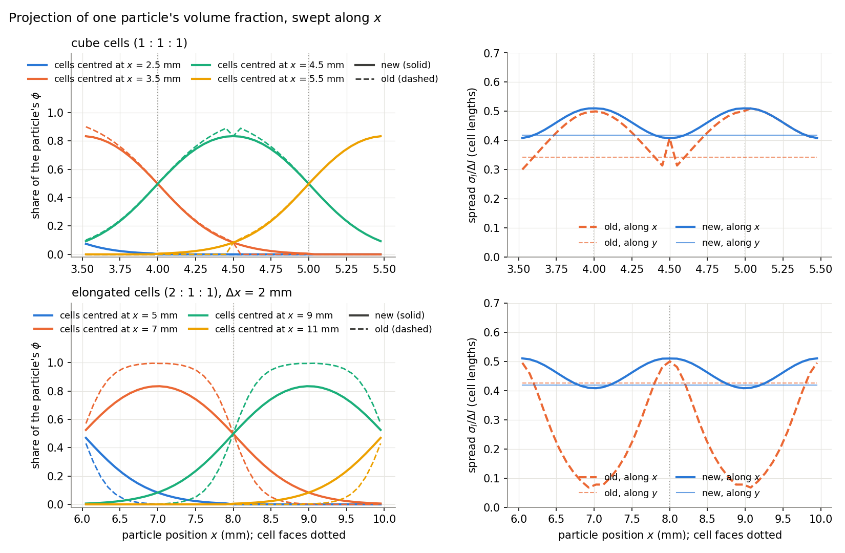
- On 2:1:1 cells the old spread along the long side fell to 0.07 cell lengths: the particle's φ landed almost entirely in one cell. The kernel now scales each direction by the receiving cell's length, and the spread stays between 0.41 and 0.51 cell lengths in every direction.
- On cube cells the old curve has a notch at the cell centre. Cells whose centre lay just outside the bin domain were dropped, so a particle reached only 8–12 cells instead of 27. The same bug made φ about 8% too high at the edge of a particle cloud.
The kernel width is still about 0.46h, so it depends on the mesh.
Low-Slip Closures
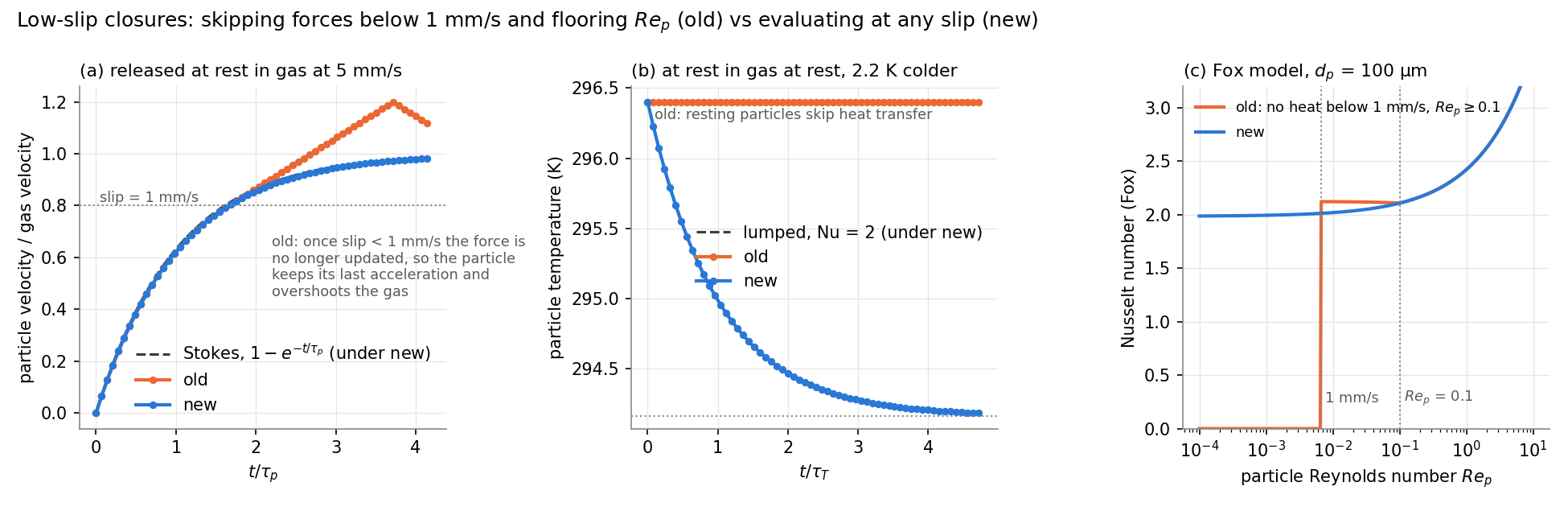
- (a) Drag. When the slip fell below 1 mm/s, the old code skipped the force update and kept its stale value. The particle went on accelerating and overshot the gas, reaching 1.2 times the gas velocity. The new code follows the Stokes solution.
- (b) Heat. A particle at rest in gas at rest exchanged no heat at all. Its temperature now relaxes as the lumped model with Nu = 2 predicts.
- (c) Fox Nusselt number. The old code gave Nu = 0 below 1 mm/s and floored Re_p at 0.1. The new formula tends smoothly to 2.
Quasi-Steady Drag
Rows 1–2: C_D from each code's Fortran routine at M → 0 and φ = 0, compared with the published correlations. Row 3: a particle released at rest in gas at 1 m/s (Re₀ = 1), compared with the ODE using the published correlation.
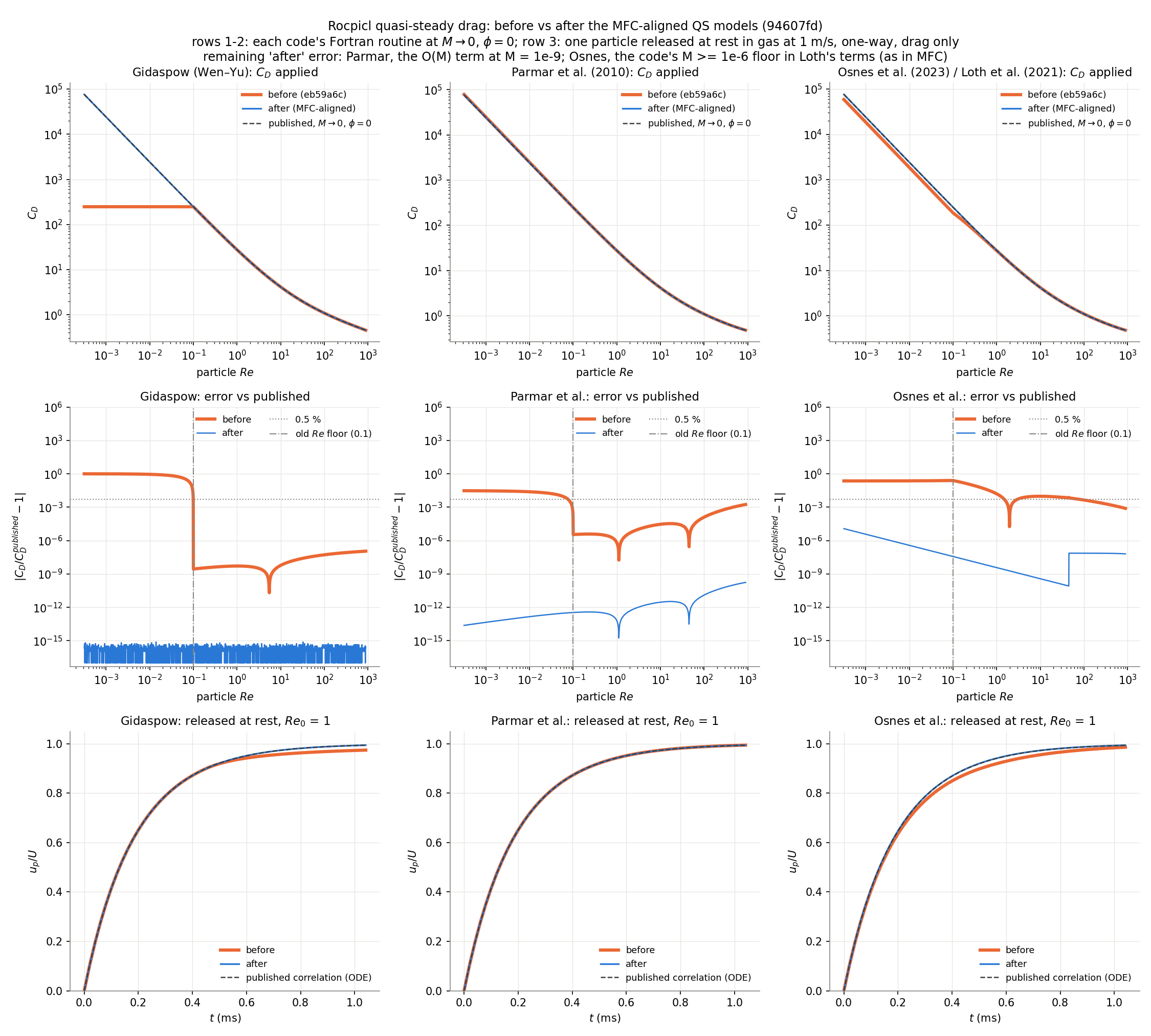
| Model | Worst error before | After |
|---|---|---|
| Gidaspow (Wen–Yu) | 100% (Re floored at 0.1 inside C_D) | 8e-16 |
| Parmar et al. (2010) | 3% | 2e-10 |
| Osnes et al. (2023) / Loth et al. (2021) | 25% (M floored at 0.01, giving a spurious Knudsen reduction) | 1e-5 |
The remaining "after" errors come from evaluating at M = 1e-9 and from the code's own M ≥ 1e-6 floor in Loth's terms. The modified Parmar model was removed.
Input decks:
QSFORCEis now 0 none, 1 Gidaspow, 2 Parmar, 3 Osnes. 4 stops with an error. Decks that usedQSFORCE 2for Osnes must change to3.
Heat Transfer: Reynolds Number in the Gunn and Sun Correlations
The convective heat rate into particle p is
Q_p = π k_f d_p (T_f − T_p) · Nu,
with Nu from the model set by HEATTRANSFER. Two of the five models were fitted to beds
of particles, and both define their Reynolds number with the superficial slip velocity:
- Gunn (1978),
HEATTRANSFER 3: Re = d U ρ/μ, with U the superficial velocity (nomenclature of the paper). For a suspension U = ε_f |u_f − u_p|. - Sun et al. (2015),
HEATTRANSFER 5: fitted to PR-DNS of random fixed assemblies against the mean slip Reynolds number Re_m = ε_f ρ_f |u_f − u_p| d_p / μ_f.
Both were evaluated with the particle Reynolds number Re_p = ρ_f |u_f − u_p| d_p / μ_f,
which is larger by 1/ε_f. Both now use Re_m (rem in ppiclf_user.f). Stokes,
Ranz–Marshall and Fox (HEATTRANSFER 1, 2, 4) are single-sphere correlations and keep
Re_p. Grawe & Capecelatro (2026) use the same definitions in their Euler–Lagrange model.
Sun's Nu is defined with the bulk (mixing-cup) fluid temperature, while the code only has the average fluid temperature. Their consistent model (eq. 29) corrects for this with the mean scaled fluid temperature ⟨θ⟩ (eq. 30):
q‴ = 6π ε_s k_f Nu / (4 d_p² ⟨θ⟩) · (T_f − T_p),
⟨θ⟩ = 1 − 1.6 ε_s ε_f − 3 ε_s ε_f⁴ exp(−Re_m^0.4 ε_s).
Divided by the number density 6ε_s/(π d_p³), this gives Q_p with Nu replaced by
π/4 · Nu/⟨θ⟩, which is what HTModel_Sun returns. That conversion was already right; ⟨θ⟩
now also uses Re_m. Sun's constants were single precision (1.4e-7 relative error) and are
now double.
The compiled HTModel_Gunn and HTModel_Sun agree with the published formulas to 4e-16
and 2e-16.
Nusselt Number against PR-DNS
The PR-DNS points (with 95% confidence intervals) are those of Sun et al. (2015) Fig. 5, read from the vector paths of the PDF. Read back the same way, the paper's own correlation curves match eq. 27 at Re_m to 0.2%, and the Gunn curve of their Fig. 4 matches Gunn at Re_m to 0.1% (3.7% with Re_p), so the paper evaluates both at Re_m.
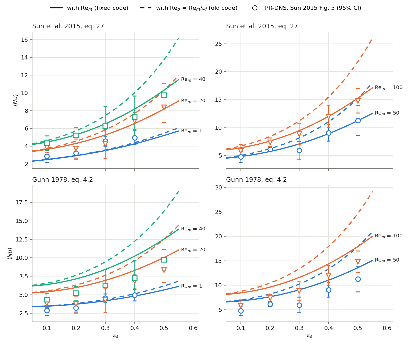
Solid lines: with Re_m (now). Dashed lines: with Re_p (before).
| Model | Re | Mean error | Largest error | Points inside the 95% interval |
|---|---|---|---|---|
| Sun | Re_m (now) | 7.9% | 24% | 23 of 24 |
| Sun | Re_p (before) | 20.9% | 48% | 13 of 24 |
| Gunn | Re_m (now) | 31% | 63% | 6 of 24 |
| Gunn | Re_p (before) | 47% | 79% | 4 of 24 |
Sun's 7.9% matches the "about 7%" the paper gives. Gunn's correlation overpredicts this PR-DNS by 20–60% even with Re_m (as in Sun's Fig. 4); Re_p added another 10–40%.
Mean Scaled Fluid Temperature
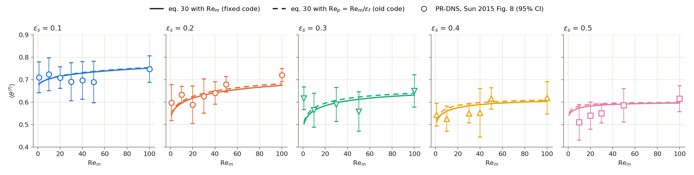
PR-DNS points from Sun et al. (2015) Fig. 8. Eq. 30 is within 5.0% of them on average with Re_m (the paper gives 5%) and 5.4% with Re_p; 27 of 30 points lie inside the 95% interval. Re only enters ⟨θ⟩ through exp(−Re^0.4 ε_s), so Re_m against Re_p changes it by 2% at most: almost all of the old error came from Nu.
Heat Rate in a Run
A periodic 8 mm box with 13,824 particles fixed on a lattice (3 × 3 × 3 per cell, so ε_s
is uniform), held at 394 K with VELOCITYMODEL 0, in gas at 294 K moving at Re_m = 50.
The gas energy gain rate over 1e-7 s is compared with N·Q_p from the published formulas:
| Model | ε_s | Run / formula with Re_m | Run / formula with Re_p |
|---|---|---|---|
| Gunn | 0.1 | 0.9973 | 0.968 |
| Sun | 0.1 | 0.9973 | 0.963 |
| Gunn | 0.3 | 0.9970 | 0.883 |
| Sun | 0.3 | 0.9970 | 0.879 |
The remaining 0.3% shrinks with the length of the run (0.16% over 2e-7 s, 0.14% over 4e-7 s): it is a fixed start-up loss of about a quarter of a time step plus the gas warming, which lowers T_f − T_p. With those two removed the run matches the formulas to 1e-4. The per-particle rate, projected to the cells, gives back the volumetric rate of the paper.
The shocktube/two-way/heat-transfer golden (Gunn) was refreshed; its four particles sit
where ε_f ≈ 1, so it changed by less than 1e-5 of each field's maximum.
Heat Transfer: Sun's Correlation in Dilute Regions
Sun et al. (2015) fitted their correlation for 0.1 ≤ ε_s ≤ 0.5 and 1 ≤ Re_m ≤ 100. Below ε_s = 0.1 the code extrapolated it, and it reaches the wrong single-sphere limit.
The π/4 in π/4 · Nu/⟨θ⟩ is not a cell-to-particle factor. Sun's heat transfer coefficient is per unit perimeter of plane sections through the spheres (Sun's thesis, eq. B.13), and for random plane sections the perimeter per unit section area is π/4 times the sphere surface per unit volume (Appendix D). So π/4 · Nu is the usual Nusselt number per unit sphere surface. As ε_s → 0, ⟨θ⟩ → 1 and
π/4 · Nu → π/4 · (2 + 0.17 Re_m^0.7 Pr^1/3),
which is π/2 at Re_m = 0 instead of 2. Against Ranz–Marshall it is 33% low at Re_m = 1 and 41% low at Re_m = 50.
From ε_s = 0.1 up, nothing changed. Below 0.1, HTModel_Sun holds Sun's value at
ε_s = 0.1 (same Re_m) and blends it into Ranz–Marshall (HEATTRANSFER 2, with Re_p):
Nu = w Nu_RM + (1 − w) Nu_Sun(ε_s = 0.1), w = 1 − 3s² + 2s³, s = ε_s/0.1.
Nu is continuous, but its slope jumps at ε_s = 0.1, where Sun's Nu rises with ε_s and the blend is flat. For Re_m ≳ 3, Nu at ε_s = 0 is above Nu at 0.1, so a curve that also matched the slope would have to dip 4–8% below Sun's value just under 0.1. The kink is the smaller error. Blending into Gunn instead dips 19–26%.
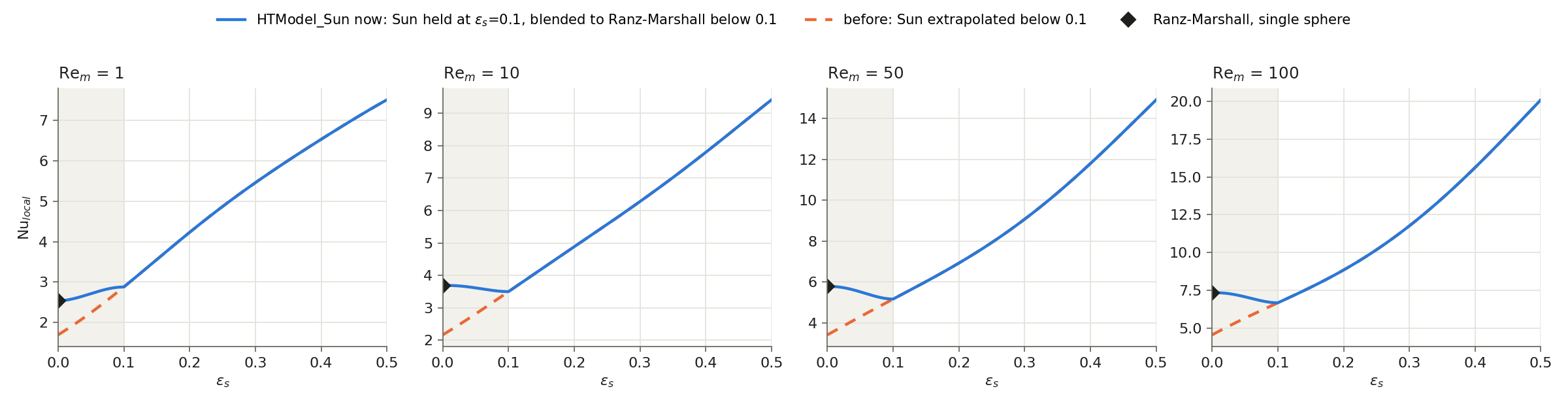
This is a modelling choice: no data fixes Nu between a single sphere and ε_s = 0.1.
Mean Temperature Decay against PR-DNS
Zhou et al. (2024, Fig. 7) give PR-DNS of the axial decay rate λ_m of the mean fluid temperature in a fixed bed down to ε_s = 0.01. Their eq. 28 makes λ_m proportional to ε_s Nu, so these points test Nu below 0.1.
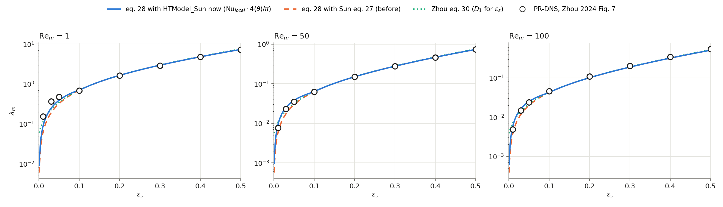
Mean error against the 24 PR-DNS points (Re_m = 1, 50, 100):
| Nu in eq. 28 | ε_s < 0.1 (9 points) | ε_s ≥ 0.1 (15 points) |
|---|---|---|
HTModel_Sun now |
18.7% | 3.1% |
| Sun extrapolated (before) | 29.3% | 3.1% |
| Zhou's fit (D₁ in place of ε_s, their eq. 30) | 23.6% | 3.6% |
Below 0.1 the new model is still low at Re_m = 1 (0.57–0.82 of the PR-DNS) and high at ε_s = 0.01 for Re_m ≥ 50 (1.20–1.22). Turning these λ_m back into Nu is not reliable below ε_s ≈ 0.03: eq. 28 uses ε_s, while Zhou's fit uses D₁, which is about twice as large at 0.01. So the points check the trend, not the blend's shape.
Heat Rate in a Dilute Run
The lattice box of Heat Rate in a Run with HEATTRANSFER 5 at
Re_m = 50, against N·Q_p from the blended formula:
| ε_s | Run / formula |
|---|---|
| 0.01 (blend weight on Ranz–Marshall 0.97) | 0.9974 |
| 0.05 (weight 0.5) | 0.9974 |
| 0.10 (Sun only) | 0.9973 |
The 0.3% is the same start-up loss as above. The regression case box/sun-dilute/np1
(gas at 5 m/s through 40 particles at 394 K, cell ε_s up to 0.075) covers the blend.
Random Numbers for the Stochastic Models
The quasi-steady force fluctuations (QSFLUCT 1 Lattanzi, 2 Osnes) add Gaussian noise to each particle (Box–Muller from uniform numbers).
Before: the uniform numbers came from gfortran's RANDOM_NUMBER, one generator per
rank. PICL_InitSolver seeded every rank with the same value (seed = 1), and each
rank drew in the order it visits its own particles. So:
- every rank drew the same sequence: the k-th particle of rank 0, of rank 1, of rank 2, … received identical noise, which correlates the forcing across the domain;
- which number a particle received depended on which rank held it and where it stood in that rank's list, so the same case gave different results on 1 and on 2 ranks, and a particle moving to another rank switched to a different stream;
- a restart could only continue the same streams by saving every rank's generator state, and only on the same number of ranks with particles in the same order.
Now: each particle carries its own
generator state in the rprop slot R_SEED (group qsfluct). The state starts at the
particle's line number in points.dat and advances by one splitmix32 step per draw
(ppiclf_op_UniformRandom in ppiclf_op.f). splitmix32 hashes a Weyl sequence, so
different seeds give unrelated streams: the first draws of particles 1 to 100,000 have a
correlation of −0.006 between neighbouring seeds. The state is an
integer below 2³², exact in a double, and moves with the particle like every other
rprop slot. Draws equal to 0 are raised to the smallest positive double, so log(u)
stays finite.
The advantages:
| Before | Now | |
|---|---|---|
| Noise of different particles | identical for the k-th particle of every rank | independent for every particle |
| Result on 1 vs 2 ranks | different | identical |
| Particle moving to another rank | switches to that rank's stream | keeps its own stream |
| Restart | needs every rank's generator state, same rank count | the state is in the particle's data; any rank count |
How it was checked
- The Fortran routine gives the same numbers as the reference splitmix32 formula for seeds 1–3 (six draws each).
- A cloud of 40 particles (the
box/momentum-exchangeset-up with a ±1 m/s velocity spread,QSFLUCT 2,NEIGHBORWIDTH 3e-3so the particles have neighbours) on 1 and 2 ranks: before, the fluctuation forces differed between the two runs and the particle velocities by up to 6.7e-6 m/s after 100 µs; now both runs are identical. - The suite's
shocktube/two-way/qs-fluctuationscase is unchanged: its four particles are farther apart than the neighbour width, so their granular temperature, and with it the noise amplitude, is exactly 0 in both versions. The new suite casebox/qs-fluctuations(np1 and np2, the cloud above) checks that the noise is on and that both rank counts agree; the old generator fails it.
Particle Collisions
Collisions use a soft-sphere model: overlapping particles push each other apart with a spring and a dashpot. The spring stiffness is the softer of two values:
- k₁ = m_eff (π² + ln² e) / (KSP·dt)². With this stiffness a contact lasts exactly
KSP time steps and rebounds with restitution e =
EREST(the linear spring–dashpot model). dt is the current time step, so the contact time follows dt. - k₂ = (4/3) E* √(R*) √δ, the Hertz stiffness at overlap δ, with E = 1 GPa and ν = 0.35 for every particle.
The dashpot is set from the chosen stiffness so that a linear contact rebounds with e.
Contact Stiffness from the Pair's Effective Mass
Commit: 3afd23a.
k₁ used particle i's own mass instead of the pair's effective mass m₁m₂/(m₁+m₂). With unequal masses each particle of a pair used a different stiffness (and could pick a different branch of min(k₁, k₂)), so the two contact forces were not equal and opposite. An 8:1 pair at 2 m/s kept 33% of its momentum; at 20 m/s its total momentum reversed. For equal masses k₁ was twice the intended value, and contacts lasted about 0.72·KSP steps instead of KSP.
The test case box/binary-collisions (np 1, 2, 4) collides four pairs across a bin face,
a rank border and the periodic faces. Particles start with an initial velocity, which
points.dat now accepts as material x y z dp u v w (786ecb1).
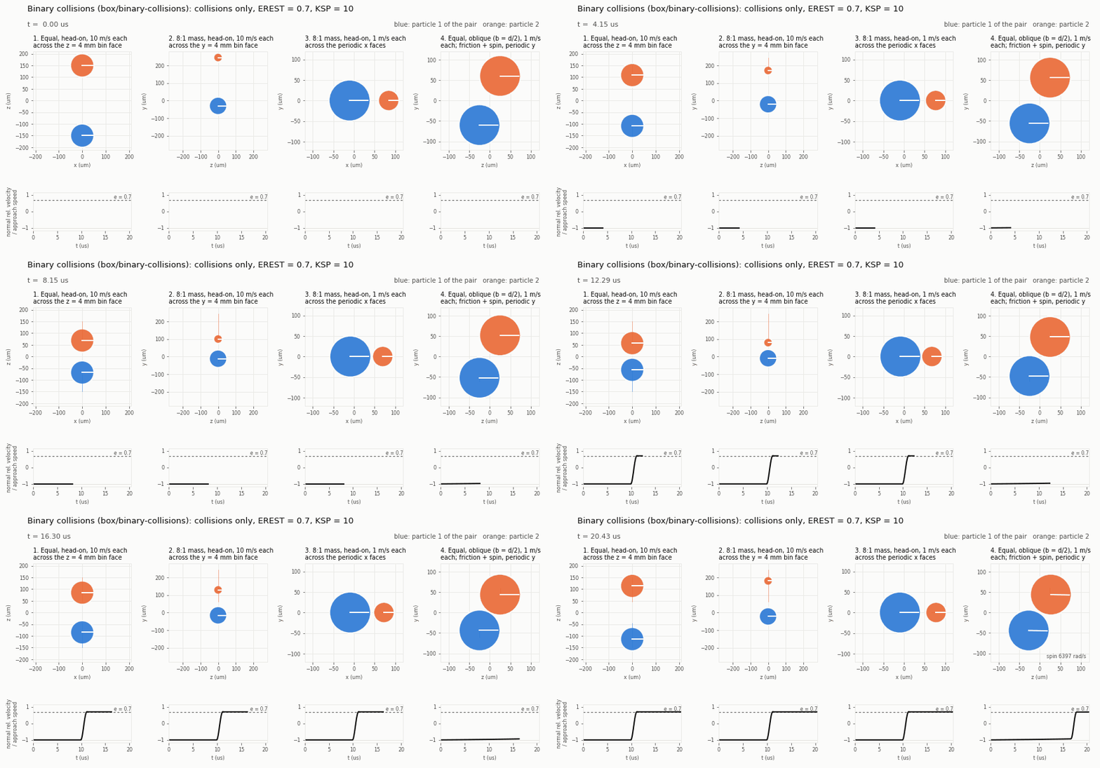
Each panel follows one pair around its centre of mass, drawn to scale, with x horizontal and y vertical (z takes the place of the missing one). The line on each particle turns with its spin. Below each panel, the normal relative velocity divided by the approach speed rebounds to e = 0.697 for the head-on pairs (EREST = 0.7). Momentum is conserved to 1e-5 and angular momentum about the centre of mass to 0.5%, including in the oblique pair (panel 4), where friction sets both particles spinning.
Ghost Particles and the Neighbour Search
Commits: f7a3980, 0bb2e4b, 82d4ca4.
A particle near a bin face is sent to the neighbouring bins as a ghost, so that pairs
across bins, ranks and periodic faces are found. The ghost algorithm was compared with
Sam's ppiclF: ghosts carry the whole state vector, velocity included. A test build whose
ghosts dropped the velocity fails the new case box/ghost-collisions on 1, 2 and 4
ranks; the current code passes it. The subbin neighbour search was compared with a brute-
force search over all real and ghost particles (scratch build) and found every pair on
1, 2, 4 and 8 ranks.
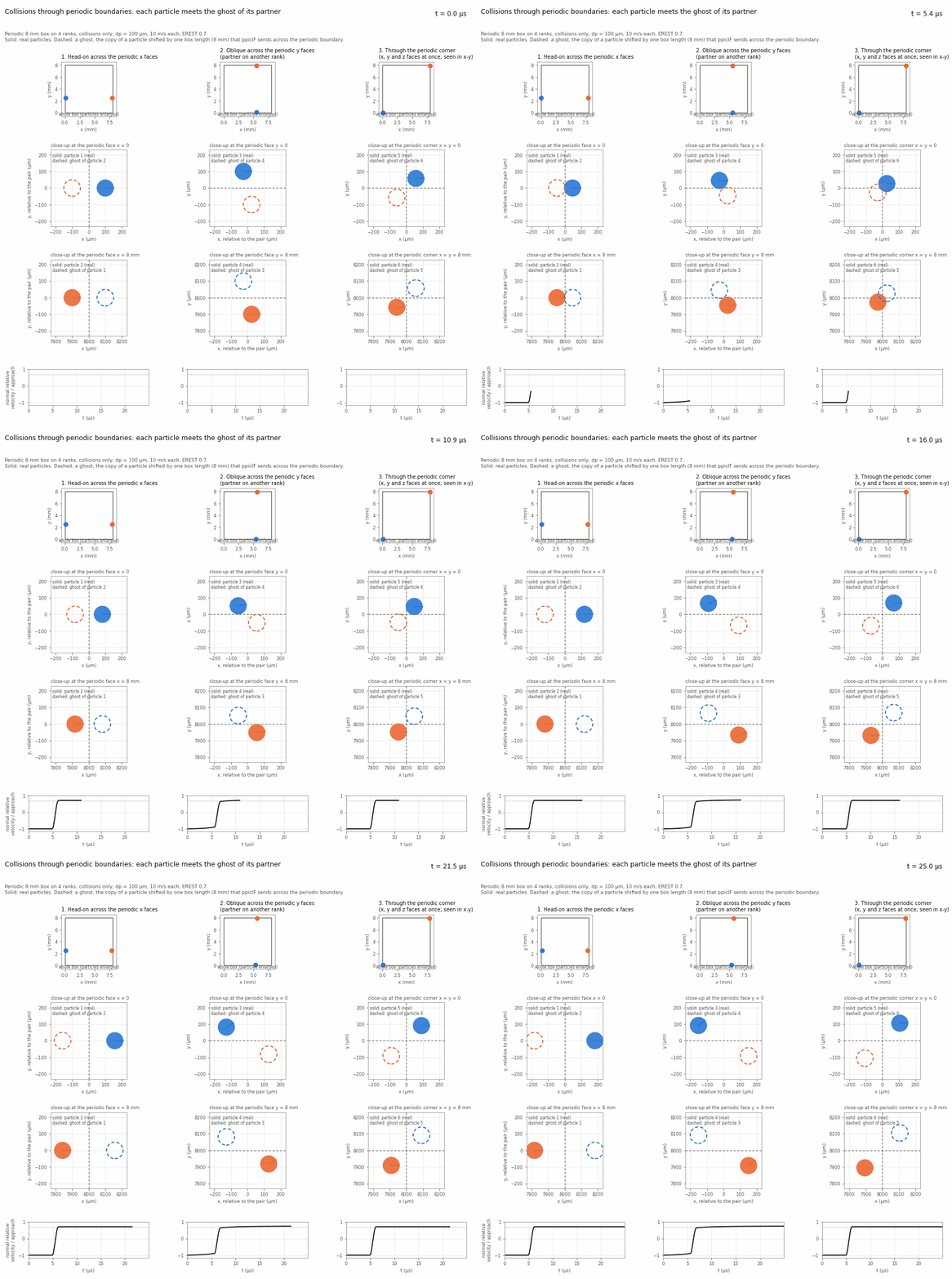
The animation shows ghosts at work in a periodic 8 mm box on 4 ranks (collisions only, 100 µm particles at 10 m/s each). Three pairs start on opposite edges of the box and collide through a periodic boundary: head-on across the x faces (both particles on one rank), obliquely across the y faces (the partner is on another rank, since the bins are split in y), and along the diagonal through the periodic corner (x, y and z faces at once). In the close-ups, each real particle (solid) meets the ghost of its partner (dashed): the partner's copy shifted by one box length. Both particles of a pair rebound with e ≈ 0.71 (the oblique pair 0.75, leaving with 66,600 rad/s of spin), and each pair's momentum is unchanged.
Two robustness fixes came with this:
- Sending or receiving more ghosts than
PPICLF_LPART_GPwrote past the end of the ghost arrays. The run now stopped with a message; since e227f99 the ghost arrays grow instead (see Memory). Ghosts no longer carry the projection values, which shrinks the ghost arrays by 30% (about 520 to 360 MB per rank at LPART = 80000). - The subbin contents were dense tables of (subbins × particles) 4-byte integers. A 2 cm bin with 0.4 mm subbins has 140,608 subbins, so 50,000 particles requested about 28 GB per call. They are now compact lists: one start index per subbin plus three integers per particle, about 1.2 MB for the same bin (12 bytes more per ghost), about 24,000 times less. The interpolation stencil search had the same kind of table over cells, which grew with the square of the cells per bin; it uses the same lists now. Results are byte-identical.
Particle–Wall Collisions
Commit: 2ff0cd8.
Turning Walls On
A slip-wall or no-slip-wall section of the .bc file with PARTWALL 1 makes that patch
a particle wall:
# BC_SLIPW
PATCH     1 2
NAME      SlipWall
PARTWALL  1     ! particles collide with these patches (default 0)
#
Patches without the key, and periodic patches, are not particle walls, so periodic runs
are unchanged. At start-up every rank gets every face of these patches, with
quadrilaterals split into two triangles. Their normals come from Rocflu and point into
the fluid. At start-up the code prints how many triangles came from which patches, and
warns if COLLISIONS is 0 (the walls then have no effect).
filein.vtk is no longer read, and a run that finds one in its directory stops with a
message. Its triangles had no known fluid side (in the cone file, for example, half of
them point each way), it had to be kept consistent with the mesh by hand, and walls that
the gas sees are exactly the fluid mesh walls. A deck that used it needs PARTWALL 1 on
its wall patches instead.
What Changed
- Same force law as pairs. The pair contact force is now one routine
(
ppiclf_user_ContactForce) used by pairs and walls. The wall is a partner of infinite mass and radius at rest: m_eff = m, R* = r, same E, ν, EREST, KSP, friction and rolling torque. Pair results are byte-identical to before. The old wall branch had its own Hertz constant (√2 too soft for a wall of the same material), no ln² e term in k₁, no friction, and started the contact 0.05·dp before the particle touched the wall. - Closest point on each triangle. The old search projected the particle onto each triangle's plane and accepted the triangle if the projection was inside it (with 10% slack). Near the edge between two triangles both accepted it, and the particle was pushed twice. The contact now uses the closest point on each triangle (face, edge or vertex). Repeated contacts are dropped, so a flat wall made of many triangles acts as one surface, and edges and corners between walls are handled.
- A fluid side. A patch wall pushes a particle back towards the fluid even when the
particle's centre has crossed the wall. The old wall turned its normal towards whichever
side the centre was on, so once the centre crossed, the wall pushed it out of the domain.
This assumes that the solid behind a
PARTWALLpatch is at leastNEIGHBORWIDTHthick (at least 4 diameters), which holds for the boundary of the fluid domain. - Search. Wall triangles are filed into the collision subbins of each rank, so a particle only checks the triangles near it. The old code checked every wall for every particle.
- Particles just outside the domain. ppiclF cut its bins back to the fluid domain's extent in every direction. A particle whose centre was briefly outside the domain was in no bin: it was dropped on 2+ ranks, and on 1 rank the subbin index went below 0 and the run crashed. Bins are now only cut back in periodic directions.
Results
The probe below fires particles (dp = 100 µm, COLLISIONS 1, EREST 0.7, KSP 10) at the
walls of a closed 8 mm box with gas at rest. The gas CFL sets dt ≈ 1.9e-7 s, so a contact
governed by k₁ lasts about 1.9 µs. The old code reads the walls from a filein.vtk of the
box (two triangles per face); the new code uses the box's slip walls with PARTWALL 1.
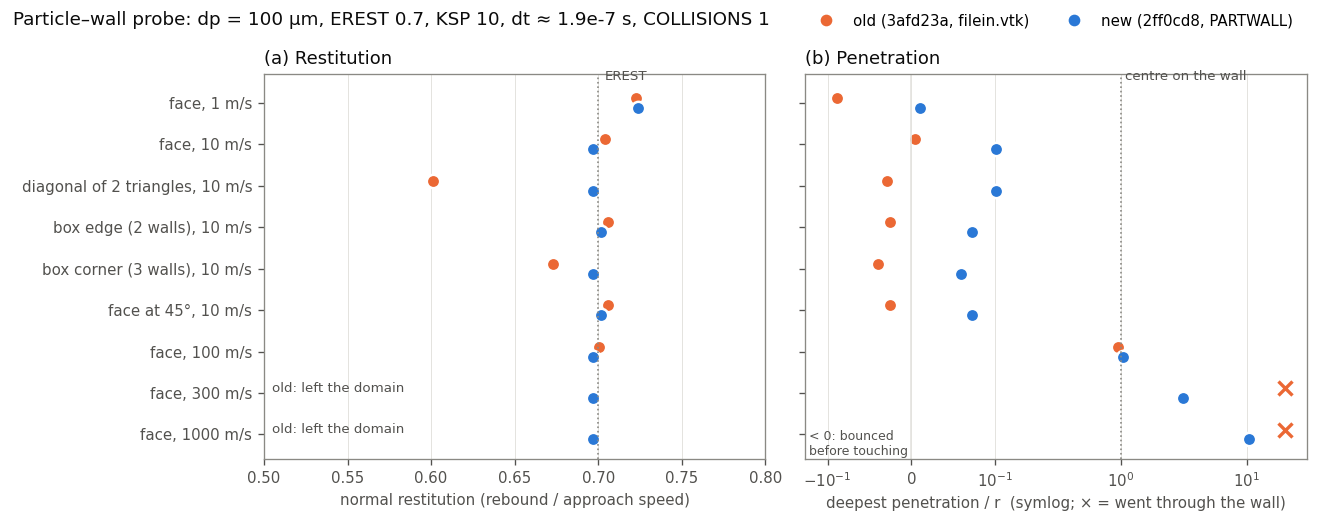
- (a) The new code rebounds with e = 0.697 on faces, on the diagonal between two triangles, at a box edge and in a corner, the same value as a head-on pair. At 1 m/s the Hertz stiffness is the softer one and e = 0.724. The old code gave 0.60 on the diagonal and 0.67 in the corner, where triangles pushed twice.
- (b) At 100 m/s the centre reaches the wall plane (penetration 1.0 r). At 300 and 1000 m/s the old wall let the particle through and the run crashed; the new wall pushes it back from 3.1 r and 10 r behind the wall, with the same e.
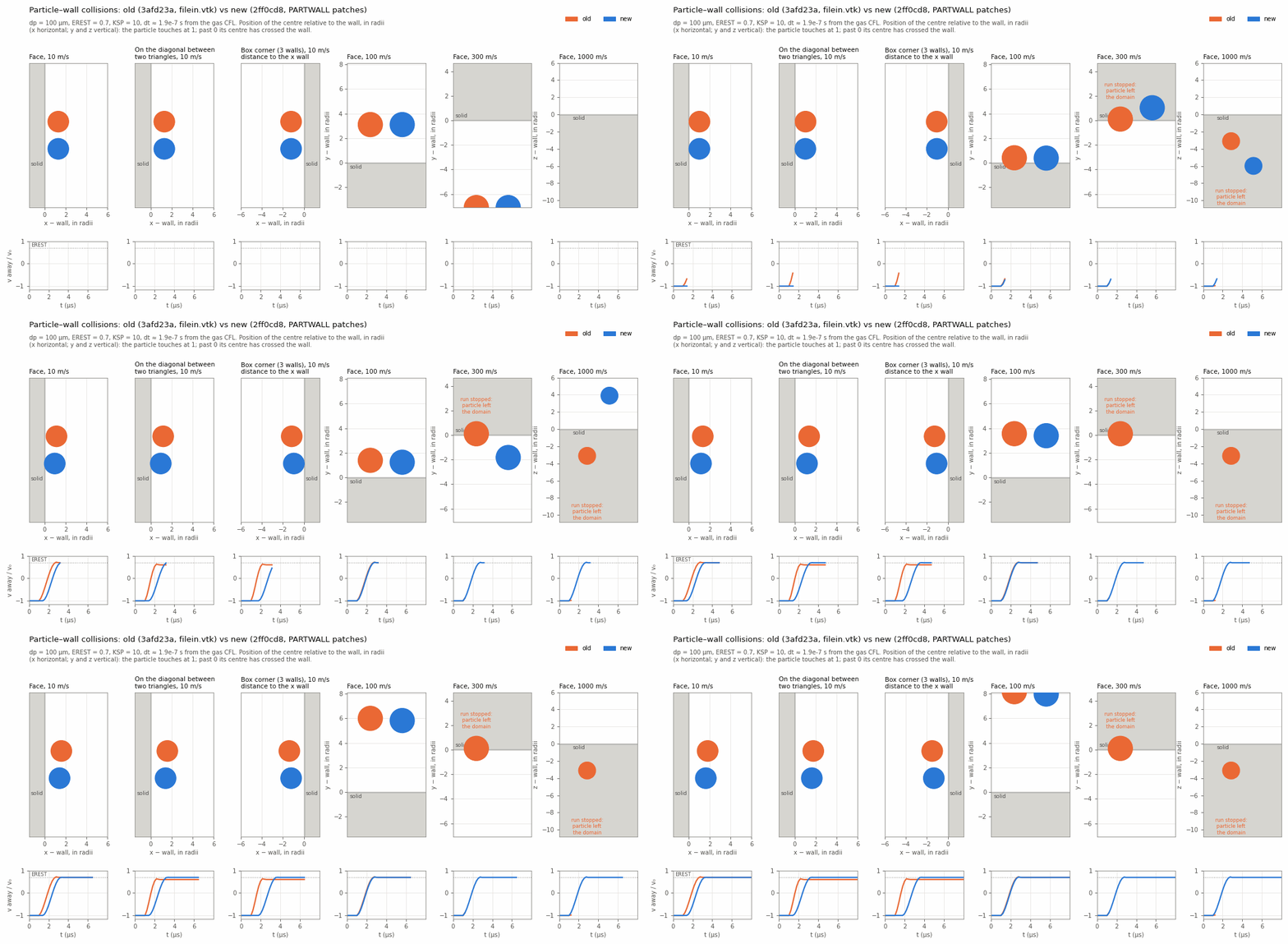
Each panel looks along the wall. The axis normal to the wall is the position of the particle's centre relative to the wall in radii (horizontal for the x walls, vertical for the y and z walls): the particle touches at 1 and its centre has crossed the wall past 0. Old (orange) and new (blue) particles are drawn to scale side by side, and the strip below shows the velocity away from the wall over the approach speed. One frame is one time step.
How deep particles go. With the k₁ stiffness the deepest penetration is about v·KSP·dt/π, whatever the material: about 3.7 r for a 100 µm particle at 300 m/s with KSP 10 and dt = 1.9e-7 s. The new wall recovers such particles, but the contact is not resolved in any physical sense. Keeping v·KSP·dt/π well below the radius needs a smaller KSP or a smaller time step. Rocflu's time step does not take particle speeds into account.
The test case box/walls (np 1, 2, 4) runs eight such shots with COLLISIONS 2 (friction
and spin). Each particle that hits one wall must rebound with e within 0.035 of EREST,
every particle must end inside the box, and 2 and 4 ranks must match 1 rank. The old code
fails it: the 300 m/s particle leaves the domain and the run crashes. At an edge or a
corner each wall's friction also slows the motion towards the other walls (e ≈ 0.55 at
the edge, 0.47 in the corner with μ = 0.4), so there the test only checks the rebound.
Memory: ppiclF Arrays Sized at Run Time
Commits: c1ac692, 0d4d86c, e227f99, 074d58d.
The Problem
ppiclF kept its data in Fortran COMMON blocks whose sizes were fixed when the code was
compiled, in libpicl/user_files/PPICLF_USER.h:
| Setting | Value | What it sized |
|---|---|---|
PPICLF_LPART |
80,000 | Particles on one rank: the state y, rprop, feedbk, iprop, the neighbour-search copy and the send buffer for particles changing rank |
PPICLF_LPART_GP |
8 × LPART = 640,000 |
Ghost particles on one rank |
PPICLF_LEE |
120,000 | Fluid cells on one rank, and cells overlapping one rank's bins |
PPICLF_LWALL |
50,000 | Particle-wall triangles |
PPICLF_VU |
50 | Steps of viscous-unsteady history per particle (500 values each, stored three times) |
Every rank reserved all of it, whatever the run needed, and the zeroing at start-up touched every page:
- A shock-tube run with one particle on 640 cells used 1.34 GB of memory (peak
resident set). The viscous-unsteady history alone took about 900 MB of it, even with
VISCOUSUNSTEADY 0. - A rank that needed more than the fixed sizes stopped ("Increase LPART", "increase PPICLF_LPART_GP", "Increase LEE"), and the code had to be recompiled.
- With
PPICLF_VU 0(to save memory) andVISCOUSUNSTEADY 1in the input, the history routines wrote past the end of zero-length arrays. - One limit was not checked at all: when a rank's bins overlapped more than
PPICLF_LEEfluid cells, the extra cells were dropped on receive without a message (see below).
What Changed
The change was made in three steps, each built and run through the whole regression suite twice before the next one:
- c1ac692: the viscous-unsteady history. The history arrays and
rprop3(the same history packed per particle, so that it moves with a particle that changes rank) became allocatable, in moduleppiclf_unsteady(ppiclf_unsteady.f). They are allocated at start-up only whenVISCOUSUNSTEADY ≥ 1, with as many steps as the new PICL keyVUSTEPS(default 50, the oldPPICLF_VU).PPICLF_VUandPPICLF_LRP3are gone.DU HEATTRANSFERis computed in the same routines, so it now needsVISCOUSUNSTEADY ≥ 1; before, it was silently zero without it. - 0d4d86c: move the arrays into a module. Every array sized by
LPART,LPART_GP,LEEorLWALLmoved from the COMMON blocks (PPICLF_SOLN.h,PPICLF_PARALLEL.h,PPICLF_GRID.h,PPICLF_GEOM.h) into moduleppiclf_data(ppiclf_data.f) as an allocatable array. Every routine that includesPPICLFgot ause ppiclf_dataline. The sizes were still the old fixed values, so this step changed only where the memory lives; results were bit-for-bit the same. - e227f99: size from the run, and grow. The fixed sizes are gone. Each group of
arrays has a capacity (
ppiclf_maxpart,ppiclf_maxghost,ppiclf_maxcell,ppiclf_maxfv,ppiclf_maxwall) that starts at 1 and grows whenever a count would exceed it.
The modules and allocatable arrays are standard Fortran 90; the files stay in fixed form
(72 columns), which gfortran compiles as before. The module files (.mod) are written to
libpicl/build/.
How the Arrays Grow
The number of particles on a rank changes during a run: ppiclF assigns particles to ranks by spatial bins, and a cloud that is compressed or swept downstream piles into fewer bins. The counts only go up in a few places, and each one now makes room first:
| Count | Where it grows | How |
|---|---|---|
| Particles | AddParticles (start-up), the restart reader, MoveParticle (particles changing rank) |
ppiclf_data_GrowPart, which also grows the viscous-unsteady history |
| Ghosts | CreateGhost (ghosts to send), MoveGhost (ghosts received) |
ppiclf_data_GrowGhost |
| Cells overlapping the bins | MapOverlapGrid (cells to send and received), the interpolation and projection transfers |
ppiclf_data_GrowCell |
| Fluid cells of this rank | InitOverlapGrid |
ppiclf_data_GrowFV, exact: Rocflu passes its cell count |
| Wall triangles | AddWall |
ppiclf_data_GrowWall |
A capacity grows to what is needed, and by at least 1.5 times, so a count that creeps up reallocates rarely (from 1 to 100,000 takes about 30 steps over a whole run). Growing copies the existing entries into the larger array; it never shrinks.
Transfers between ranks. Particles, ghosts and cells move between ranks through
gslib's crystal router. If a rank receives more than its arrays hold, the router keeps what
fits, drops the rest, and only reports the full count afterwards; growing after the
transfer would be too late. So before each of the five transfers, ppiclf_comm_NumIncoming
counts the columns each rank sends to each other rank and adds them up with one
MPI_Reduce_scatter_block, which tells every rank how many it will receive. The rank grows
its arrays to that number, then the transfer runs. Each transfer still checks the received
count afterwards, as a guard that should never trigger.
Restart. The particle reader used to fill the first ranks with PPICLF_LPART
particles each. It now gives every rank an equal block, ⌈total / ranks⌉, the same split
Rocflu uses for points.dat; ppiclF then moves the particles to the ranks that own their
bins, as before. (Restart itself is still unverified; see Still open.)
Two Bugs Found on the Way
- Cells dropped without a message (
MapOverlapGrid). Only the number of cells a rank sent was checked againstPPICLF_LEE; the number it received was not. A rank whose bins overlapped more than 120,000 fluid cells lost the extra cells, so particles near them interpolated from, and projected onto, an incomplete stencil. Now the cell arrays grow before the transfer. points.datread one column past the rank's share (PICL_InitSolver). Every line ofpoints.datis read on every rank, to get the global bounding box, but the position was read straight into the rank's particle buffery(:,i). Once a rank had its share, the remaining lines went into columnnpart_local + 1. That was harmless while the buffer had 80,000 columns; with a buffer of exactly the rank's share it corrupted memory and the 2- and 4-rank cases crashed at exit. The position is now read into a local variable and copied only for the rank's own particles. Valgrind found this one.
How It Was Checked
- Regression suite: 35 PASS, twice, after each of the three steps, with the goldens unchanged. Since every capacity starts at 1, every case grows its arrays many times (on 1, 2 and 4 ranks, with ghosts across ranks and periodic faces), so the growth paths are covered by the whole suite.
- Valgrind on
box/ghost-collisions/np4andbox/walls/np4(4 ranks, ghosts growing and moving between ranks): no invalid reads or writes. - Beyond the old limit: 120,000 particles on one rank (the old limit was 80,000) run to the end, and all 120,000 are in the particle output.
- Memory, shock tube with one particle on one rank (peak resident set):
| Build | Memory |
|---|---|
| Before (fixed arrays, 50-step history) | 1,342 MB |
c1ac692 (history only when VISCOUSUNSTEADY ≥ 1) |
807 MB |
| e227f99 (everything sized from the run) | 265 MB |
Most of the remaining 265 MB is Rocflu and MPI. The fixed-size data of the solver
executable rflump (its bss segment) went from 1.8 GB to 0.5 MB. With VISCOUSUNSTEADY 1 the history is allocated as
before, per particle (about 12 kB per particle for 50 steps).
What Changes for Users and Developers
PPICLF_USER.hno longer hasPPICLF_LPART,PPICLF_LEE,PPICLF_LWALL,PPICLF_VUorPPICLF_LRP3. There is nothing to raise for a larger run.VUSTEPSin the PICL section sets the length of the viscous-unsteady history.- The spare property arrays
rprop2,rprop4,rprop5(PPICLF_LRP2/4/5, all 0) and the unused "store forces" block that wroterprop5are gone, and so isppiclf_user_InitZero: the history is allocated with the other arrays inppiclf_data_Allocateand zeroed inppiclf_solve_InitZero. - A new per-particle array goes in module
ppiclf_data: declare it, allocate it inppiclf_data_Allocate, and add it toppiclf_data_GrowPart. Routines that use it needuse ppiclf_data(every routine that includesPPICLFalready has it). - Arrays whose size is a particle, ghost or cell count must not be given a fixed size anywhere else (local buffers included): size them from the current count or capacity.
- The number of entries per particle or cell is set at run time too; see the next section.
Field Sizes Set at Run Time
The three steps above size each array's particle, ghost, cell or wall dimension from
the run. The other dimension, how many entries a particle or a cell carries, was still a
compile-time constant in PPICLF_USER.h. Rocflu had to keep its number of
InterpFieldUser calls equal to PPICLF_LRP_INT by hand. Now both dimensions of every array are set
when the run starts.
| Size | Arrays | Was | Now |
|---|---|---|---|
| State per particle | y, y1, ydot, ydotc |
PPICLF_LRS 10 |
ppiclf_lrs |
| Properties per particle | rprop, cp_map (with y) |
PPICLF_LRP 53 |
ppiclf_lrp |
| Interpolated fields | int_fld, int_fld_input |
PPICLF_LRP_INT 29 |
ppiclf_lrp_int |
| Projected fields | feedbk, pro_fld, pro_fld_picl |
PPICLF_LRP_PRO 31 |
ppiclf_lrp_pro |
| Properties a ghost carries | rprop_gp (with y) |
PPICLF_LRP_GHOST 6 |
ppiclf_lrp_ghost |
- One user routine sets them.
ppiclf_user_Layout(libpicl/user_files/ppiclf_user_Layout.f) setsppiclf_lrs,ppiclf_lrpandppiclf_lrp_pro. It lists the interpolated slots (ppiclf_solve_AddInterpSlot) and the slots ghosts carry (ppiclf_solve_AddGhostSlot).PICL_InitSolvercalls it once throughppiclf_solve_InitLayout, after the PICL flags are read and before any particle exists, and gets back the sizes ofyandrpropto create the particles. Rank 0 prints the sizes and both lists. - ppiclF counts the interpolated fields itself. The count is the length of the
list. The check in
PICL_Runge*.F90that the number of fields was 29 is gone. Instead ppiclF stops with the slot number if, in a stage, Rocflu gives a slot that is not on the list, gives one twice, or leaves one out. (At start-up ppiclF interpolates once before Rocflu has given any field; then nothing is interpolated, as before.) - The slot lists are module arrays.
ppiclf_int_slotsreplacesPPICLF_INT_MAP, which was kept in a COMMON block and filled in call order. A field's column is now its place in the list. Each field is interpolated on its own, so the order changes no result. - Removed macros:
PPICLF_LRS,PPICLF_LRP,PPICLF_LRP_INT,PPICLF_LRP_PRO,PPICLF_LRP_GHOST,PPICLF_GHOST_SLOTS_INDEX,PPICLF_LRP_GP,PPICLF_INTERP,PPICLF_PROJECT. The slot names (PPICLF_J*,PPICLF_R_*,PPICLF_P_*) stay. - Local arrays sized by these numbers (the neighbour routine's
yi,rpropi,yj,rpropj) are sized from the module variables, so-fcheck=allstill checks them.
In 074d58d the layout is the one the macros gave: every field on. Checked: in all cases (the suite and model variants) every particle and flow file is byte-identical to f4d6486; 35 PASS twice.
Only the fields the physics needs
With the sizes set at start-up, ppiclf_user_Layout now reads the PICL flags and keeps
only the fields that a model that is on uses.
Interpolated gas fields: before, all 29 were sent between ranks and interpolated to every particle at every RK stage.
| Gas fields at the particle | Interpolated when | Read by |
|---|---|---|
| ρ_g, φ_p, u_g, c_g, T_g (7) | always | drag, heat transfer, viscosity, every model |
| ∇p (3) | PGFORCE 1 or AMFORCE 1 |
pressure-gradient force, Parmar added mass |
| Du/Dt, ∂(ρφ_g)/∂t, ∇(ρφ_g), ∇ρ (10) | AMFORCE ≥ 1 or VISCOUSUNSTEADY ≥ 1 |
added mass, viscous unsteady force |
| vorticity, Dω/Dt (6) | COLLISIONS ≥ 2 |
torque, lift |
| ∇·τ (3) | PGFORCE 1 with the Navier–Stokes flow model |
pressure-gradient force |
A run with drag only interpolates 7 fields. Rocflu still computes all 29 and hands each
over; InterpFieldUser ignores a field that is not on the list. ppiclF still stops if a
field on the list is not given in a stage. A slot that is not interpolated stays zero, so
a model that starts reading a gas slot must have it added to the list.
Projected fields: 10 instead of 31 (φ_p, force, energy, and the five fields the probes read
in WriteProbe.F90).
Particle output: GRADGAS_WRT 1 writes only the gradient fields that were interpolated (the
others would be zeros). The regression harness now reports a field that is in a golden but
no longer written as a failure, instead of stopping with an error.
Checked: the suite and model variants. Against 074d58d the flow files are byte-identical and every particle field that is still written is bit-identical; the fields no longer written are exactly the ones the table leaves out for each case. The 32 goldens with particles were regenerated: all 7,641 values they share with the old ones are unchanged; ∇p is gone where no model uses it; and spin (zero) was added where a golden predated spin in the harness's field list. Not run: the ∇·τ branch (a Navier–Stokes shock tube stops in Rocflu's start-up, with or without this change).
Still to do: rprop and y keep all their slots (temperature without HEATTRANSFER, spin
without COLLISIONS ≥ 2). Dropping them changes slot
numbers from run to run, which Rocflu, which knows them only as compile-time constants,
would need to follow.
Particle Properties (rprop)
ppiclf_rprop(:, i) holds everything about particle i that is not in the state
y. It had 59 slots doing four different jobs, in no particular order, and all of them
moved with the particle, went to every ghost, were written to every par*.vtu file (as
rpro01 to rpro59) and were read back on restart. Before the changes below:
| Job | Slots (old numbering) | Needed |
|---|---|---|
| Particle properties | 1 ρp, 3 dp, 4 Vp, 22 superparticle loading | Every step, and on restart. Set once in PICL_InitSolver |
| Carried from step to step | 25–27 quasi-steady force fluctuation | Every step, and on restart: each step updates the previous value |
| Gas values at the particle | 2, 5–19, 24, 31–33, 36–45 (30 slots) | During the step only: Rocflu interpolates them before every stage. Slot 36 (gas pressure) is never read |
| Read from neighbours | 28–30 Ẇ | Added mass (AMFORCE 2) reads it from neighbouring particles, ghosts included |
| Diagnostics | 23 (|v|) | Output only |
| Unused | 20 (never written), 21 (written from a hard-coded 50 µm, never read), 34, 35 (freed when the burn-rate model was removed) |
Planned, one commit at a time:
- Ghosts carry only what the neighbour search reads (done, below).
- Choose the fields of the particle output with a list, and name them (done, below).
- Remove the unused slots and group the rest by job (done, below).
- A double-precision particle dump (
restart_data/particles_<step>.dat) holding the state a run needs to continue (done). Ofrpropit holds the slots a restart needs, listed inppiclf_user_Layoutwithppiclf_solve_AddRestartSlot(properties, quasi-steady fluctuation and its random-stream state, added-mass Ẇ), and the slots of the particle output; the gas values at the particle are interpolated again before every stage. The suite's restart test shows that this is enough: a restarted run ends byte-identical to one that never stopped.
Ghosts Carry Only What the Neighbour Search Reads
Commit: a7f5748.
A ghost carried y and all of rprop: 69 doubles. The neighbour routine
(ppiclf_user_EvalNearestNeighbor) reads only dp, ρp, Vp and Ẇ from its neighbour, so a
ghost now carries y and those 6 slots: 16 doubles, 128 bytes instead of 552, in memory
and in the ghost transfer.
- The slots are listed once. They were macros in
PPICLF_USER.h(PPICLF_LRP_GHOST,PPICLF_GHOST_SLOTS_INDEX); they are nowppiclf_solve_AddGhostSlotcalls inppiclf_user_Layout(see Field sizes set at run time), which fillppiclf_ghost_slots(1:ppiclf_lrp_ghost). ppiclf_comm_CreateGhostpacks those slots aftery.- The neighbour search unpacks a ghost's slots into a full-length local
rpropjbefore calling the user routine, so the routine's interface is unchanged. Slots a ghost does not carry are zero. ppiclf_cp_map, the real particles' copy, keeps all ofrprop: particlei's own values (rpropi) and the wall contacts read more than these 6 slots.- If the neighbour routine starts reading another slot from
rpropj, add anAddGhostSlotcall for it inppiclf_user_Layout. Otherwise a ghost passes zero for it, and only pairs across a rank boundary or a periodic face are wrong.
Checked: all 35 suite cases, plus AMFORCE 2 versions of the ghost-collision (1, 2 and 4
ranks) and binary-collision (2 and 4 ranks) cases, write byte-identical particle and flow
files before and after. Ẇ is non-zero in those runs, so the ghosts' Ẇ is used. The suite
itself has no AMFORCE 2 case across ranks.
What it saves
Each ghost is 584 bytes before and 160 bytes after: its reals (69 or 16 doubles) plus 8 integers
(iprop_gp: tags, bin, destination rank). That is 3.65 times less to hold and to send.
Measured on a periodic 8 mm box with a 37³ lattice of particles (50,653 particles,
dp = 100 µm, about 5% by volume, 16³ cells), collisions on, 155 steps (480 ghost exchanges, one per
RK stage), one 16-core node, 3 runs of each build alternating. The two builds are 74b8f87
and a7f5748 with the same temporary timers: a barrier, then CreateGhost, a barrier, then
MoveGhost, a barrier. The barriers keep a rank's wait for slower ranks out of the timers.
| Ranks | Ghosts per rank (real particles per rank) | Ghost exchange, 480 calls: before → after | Ghost data sent per rank per exchange | Ghost arrays per rank | Peak memory per rank | Whole run |
|---|---|---|---|---|---|---|
| 4 | 7,181 (12,663) | 3.0 s → 1.35 s | 4.2 → 1.15 MB | 7.1 → 1.9 MB | 209 → 200 MB | 138.6 → 135.6 s |
| 8 | 4,316 (6,332) | 3.5 s → 1.7 s | 2.5 → 0.69 MB | 3.2 → 0.86 MB | 172 → 166 MB | 86.9 → 86.1 s |
| 16 | 3,126 (3,166) | 2.9 s → 1.7 s | 1.8 → 0.50 MB | 3.2 → 0.86 MB | 164 → 160 MB | 63.5 → 62.1 s |
Times are medians of the 3 runs; the ghost exchange varied by up to ±0.6 s between runs.
- The transfer (
MoveGhost) is 2.4 to 3.2 times faster (2.25 → 0.78 s on 4 ranks), close to the 3.65 times fewer bytes. Building the ghosts (CreateGhost) changes little: it still copies all ofrpropintocp_map. The exchange as a whole takes about half the time. - The whole run is 1–2% faster, because the ghost exchange is only about 2% of this run. Most of the time is in the neighbour search, the forces and the fluid solver.
- The memory saved grows with the number of ghosts: 424 bytes per ghost the rank can hold (its capacity), plus the same again for the copies gslib makes while sending. A rank has many ghosts when its bins are small next to the neighbour distance: on 16 ranks here a rank holds about as many ghosts as real particles, and a dense production run on many ranks can hold more ghosts than real particles. For example, a rank with 10⁶ ghosts saves about 0.4 GB.
- Everything runs on one node, so the transfer is a memory copy. Across nodes the network carries 3.65 times fewer bytes, so the saving should be at least as large there.
The case and scripts are in tests/_work/bench (not tracked): bench_setup.py makes the case,
bench_run.sh runs it and analyze.py reads the GHOSTT lines the timed builds print.
Particle Output: A List of Named Fields
Being in rprop and being written to the particle files are now separate questions.
The writer (ppiclf_io_WriteParticleVTU) used to write all of y, all 59 rprop
slots and the 3 tags, as y01…, rpro01… and tag01…. It now writes the fields of
a list, built once by ppiclf_user_OutputFields (libpicl/user_files). Each entry
is a slot of ppiclf_y, ppiclf_rprop or ppiclf_iprop and the name it is written
under. A slot that is not in the list is still computed and used; it is only not
written. Positions are always written, as the points of the file.
| Group | Fields | Written when |
|---|---|---|
| Default | vp_x vp_y vp_z (particle velocity), phi_p (particle volume fraction: the projected particle volume, interpolated back to the particle), dp, id id_rank id_cycle (index on the rank that created the particle, that rank, the cycle it was created on) |
Always |
| Particle | Tp, omp_x omp_y omp_z (spin), rhop, volp |
PARTICLE_WRT 1 |
| Gas at the particle | rho_g, ug_x ug_y ug_z, c_g (sound speed), T_g |
GAS_WRT 1 |
| Gas gradients at the particle | dpdx_g …, DuDt_g_*, drhophidt_g, drhophidx_g …, vort_g_*, drhodx_g …, divtau_g_*, DvortDt_g_* |
GRADGAS_WRT 1, for checking the interpolation |
| Models | Ffluct_* (with QSFLUCT), Wdot_* (with AMFORCE 2) |
MODEL_WRT 1, for the models that are on |
- The four keys go in the
# PICLsection; all default to 0. No key is the start of another, because Rocflu'sReadSectionmatches the start of each input line (a keyGASwould also match a lineGASGRAD 1). - They were called
OUTPARTICLE,OUTGAS,OUTGRADGASandOUTMODELat first, and were renamed in the style of the fluid output keys (DENSITY_WRT, ...); the case validator tells an input with an old name what it is now. - The superparticle loading (always 1 for now) and the unused slots are not written.
- To add a field: one
call ppiclf_io_AddOutputField(source, slot, 'name')inppiclf_user_OutputFields, inside the group it belongs to. The call stops the run if the slot is out of range, the name is empty, longer than 24 characters or used twice, or the list is longer than 80 fields. - File size: each particle used to take 300 bytes per file (3 position values and 72 fields of 4 bytes); with the default fields it takes 44 bytes, 6.8 times less. For the 4-particle shock tube: 9,395 bytes before, 1,807 with the default fields and 5,860 with the three groups the regression suite turns on.
Particle restart stops for now. A restart used to read y and all of rprop back
from the last par*.vtu file, in file order. The files now hold only the output fields
(in single precision, which a restart should not use anyway), so a restart stops at
start-up with "Particle restart is not available yet" until the separate restart file
exists. A new run (no .rin file) is unaffected.
Regression suite. The template input turns on PARTICLE_WRT, GAS_WRT and
GRADGAS_WRT, so the goldens keep checking the same quantities (the gradients only where a
model needs them; see Only the fields the physics needs). The harness and the 32
goldens with particles use the new names; the conversion renamed keys only (8,790
values compared, none changed) and dropped the superparticle loading, which was 1.0 in
every golden. Checked: in all cases with particles (the suite and model variants), every named field is bit-identical to the
field it replaces in the files of 74b8f87 (e.g. rho_g to rpro02), and the flow
files are byte-identical. The default output alone and MODEL_WRT with QSFLUCT were also run.
Unused Slots Removed, the Rest Grouped by Job
Six unused rprop slots and one interpolated field were removed. The PPICLF_R_* names
are unchanged; only their numbers moved, so each job is one block (PPICLF_USER.h):
| Job | Contents |
|---|---|
| Particle properties | JRHOP, JDP, JVOLP, JSPL |
| Model state carried from step to step | FLUCTFX/Y/Z, WDOTX/Y/Z |
| Gas at the particle, interpolated every stage | JRHOF, JPHIP, JUX/Y/Z, JCS, JT, JDPDX/Y/Z, JSDRX/Y/Z, JRHSR, JPGCX/Y/Z, JXVOR/Y/Z, JRHOGX/Y/Z, JDPVDX/Y/Z, JSDOX/Y/Z |
Removed:
JDPi(never written) andJDPe(rewritten every step as 50 µm/|v| × dp, a leftover "axisymmetric collision correction" that nothing read).JSPT, the particle speed |v| stored "for plotting"; it only fedJDPe. ParaView computes it fromvp_x vp_y vp_z.JP, the gas pressure: Rocflu computed it and ppiclF interpolated it every stage, and nothing read it. Its array (ppF) and itsInterpFieldUsercall are gone fromPICL_Runge.F90andPICL_Runge_EulerPT.F90. (The check there that the number of interpolated fields was 29 has since been replaced by ppiclF's own check; see Field sizes set at run time.)- Slots 34 and 35, empty since the burn-rate model was removed.
Each particle now stores 48 bytes less in rprop, and the same again in the
neighbour-search copy (cp_map) and in every transfer of a particle to another rank.
One field less is computed, sent between ranks and interpolated every stage.
Adding a slot: put it in the block of its job and renumber the rest of that block
and the blocks after it; nothing in the code uses slot numbers directly, only the
PPICLF_R_* names. ppiclf_user_Layout sets ppiclf_lrp to the last slot
(PPICLF_R_RTerm2Perp) and lists the gas block PPICLF_R_JRHOF to PPICLF_R_JSDOZ as
interpolated, so a slot added inside the gas block is interpolated without further change;
Rocflu then has to hand it over with an InterpFieldUser call in both
PICL_Runge*.F90 files.
Checked: 35 PASS twice; in all cases with particles (the suite and model variants) every named field is bit-identical to the old field it replaces in the files of 74b8f87, and the flow files are byte-identical.
Particle Bins: Number of Bins per Direction
ppiclF splits the box around the particles into bins, at most one per MPI rank, and each
rank holds the particles in its bin. Particles within a filter width of a bin face are
also copied to the neighbouring bin as ghosts. Each bin must be at least BinMinLen long
in every direction (the larger of the projection filter width and the neighbour-search
width), and there can be no more bins than ranks. The bins are recomputed when a particle
leaves the previous bin box.
What Went Wrong
A particle bed that stretched along one direction stopped the run:
 correct bin combination not found
 binERROR: Num Bins > NumProcessors          35          32          32
PPICLF: ERROR (rank     0) Error in Createbins
A wedge case (a strong shock through a thin bed, 32 ranks) stopped this way just after 12 µs, when the bin box had stretched from 5.8 × 4.8 × 1.4 mm to about 36.7 × 5.8 × 1.4 mm.
The bin count used since April 2025 estimated a count per direction that gives bins close to cubes, then searched one bin more or less in each direction for a combination within the ranks. It had two bugs:
- Wrong split between two long directions. When the estimate gave too many bins, the code kept one bin in the short direction and split the N ranks between the other two as √N·L_med/L_large and √N·L_large/L_med. A split in proportion to the lengths is √(N·L_med/L_large) and √(N·L_large/L_med). For the wedge bed this gave 35.7 × 0.9 bins instead of 14.2 × 2.25; rounded to 36 × 1, and one bin less still makes 35 > 32.
- No safe fallback. When the search found no combination within the ranks, the code went on with the estimate minus one in every direction (35 bins for 32 ranks), and the check after it stopped the run.
Compiled on its own and run over 61,705 bin boxes on 8 to 128 ranks, this count failed on 7,713 (12%): 4,686 stuck in its iteration ("CreateBin stuck in infinite loop") and 3,027 as above. With the formula corrected, 4,261 still failed.
The New Count
ppiclf_comm_BinCounts (libpicl/source/ppiclf_bincounts.f, 0688f68) starts from one
bin and keeps adding a bin to the direction whose bins are longest, among the directions
where one more bin keeps the total within the ranks and the bins at least BinMinLen
long. It stops when no direction can take another bin. Every step keeps the layout
valid, so there is no failure case.
ppiclF's original count (before April 2025) also started from one bin, but added bins to x, y and z in turn, whatever the shape of the box: a stretched bed got long, thin bins and more ghost particles. Splitting the longest direction keeps the bins close to square, as the April 2025 count intended. The internal bin-face area measures how many particles are copied as ghosts:
| Bin box (mm) | Ranks | Original ppiclF | April 2025, formula corrected | New |
|---|---|---|---|---|
| Wedge bed at t = 0, 5.8 × 4.8 × 1.4 | 32 | 6 × 5 × 1, 65 mm² | 6 × 5 × 1, 65 mm² | 6 × 5 × 1, 65 mm² |
| Wedge bed at the crash, 36.7 × 5.8 × 1.4 | 32 | 6 × 5 × 1, 242 mm² | 15 × 2 × 1, 163 mm² | 16 × 2 × 1, 171 mm² |
| Slab, 40 × 40 × 4 | 64 | 4 × 4 × 4, 5,760 mm² | 8 × 8 × 1, 2,240 mm² | 8 × 8 × 1, 2,240 mm² |
| Long bed, 100 × 5 × 5 | 128 | 5 × 5 × 5, 4,100 mm² | 42 × 1 × 3, 2,025 mm² | 32 × 2 × 2, 1,775 mm² |
The original column uses ppiclF's single minimum length, the largest of the three. As committed, the April 2025 count stops on the wedge bed at the crash.
Unchanged: the bin box (the particles' extent plus a buffer, snapped to the walls),
BinMinLen, and keeping the bins while every particle stays inside the previous bin box.
How the New Count Was Checked
- Over 222,138 bin boxes on 8 to 256 ranks, the new count gives no invalid layout.
unit/bin-countsin Regression Tests (0887252) checks 10 bin boxes against fixed counts and 333,207 layouts for validity. A copy of the count with the rank limit doubled fails it.- The wedge case (slip walls, 32 ranks) runs to 20 µs, where it stopped just after 12 µs. The bins are the same as before up to 11 µs, then stay at 16 × 2 × 1 as the bed stretches to 64.8 × 6.9 × 1.4 mm.
- The 38 regression cases pass.
MPI and Periodic Boundaries
Each fix is checked by a regression case that compares 1, 2 and 4 ranks and checks the conservation budgets. The figures compare the commit before each fix with the current code, on 1, 2 and 4 ranks.
-
Stale virtual cells at rank borders (e3ed370).
PICL_InitSolverconverted the conserved variables before virtual cells had φ, and did not exchange them again. A quiescent particle cloud set the gas in motion (1e-4 m/s) on 2 and 4 ranks, and the total gas energy differed from the 1-rank run by 5e-8. φ is now exchanged before the virtual-cell state is computed in every stage.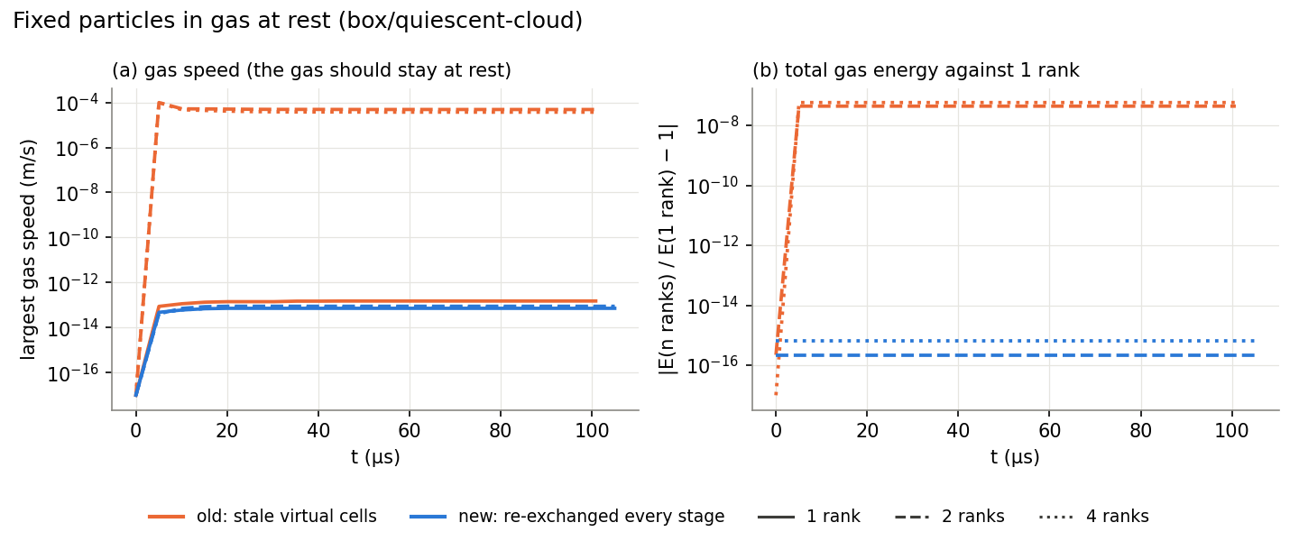
Fixed particles in gas at rest (
box/quiescent-cloud). Before the fix the gas on 2 and 4 ranks reached 1e-4 m/s and its total energy differed from the 1-rank run by 5e-8; on 1 rank, with no rank border, the gas stayed at rest. Now every rank count stays at rest (below 1e-13 m/s) and agrees with 1 rank to 6e-16. -
Periodic and symmetry patches (11dc640). Virtual cells used their own gradients, so the fluxes through these patches did not cancel. Gradients are now exchanged (
RFLU_MPI_ExchangeGradCells) and transformed (RFLU_RELP_TransformGradWrapper), so every virtual cell uses the gradient of the real cell it mirrors.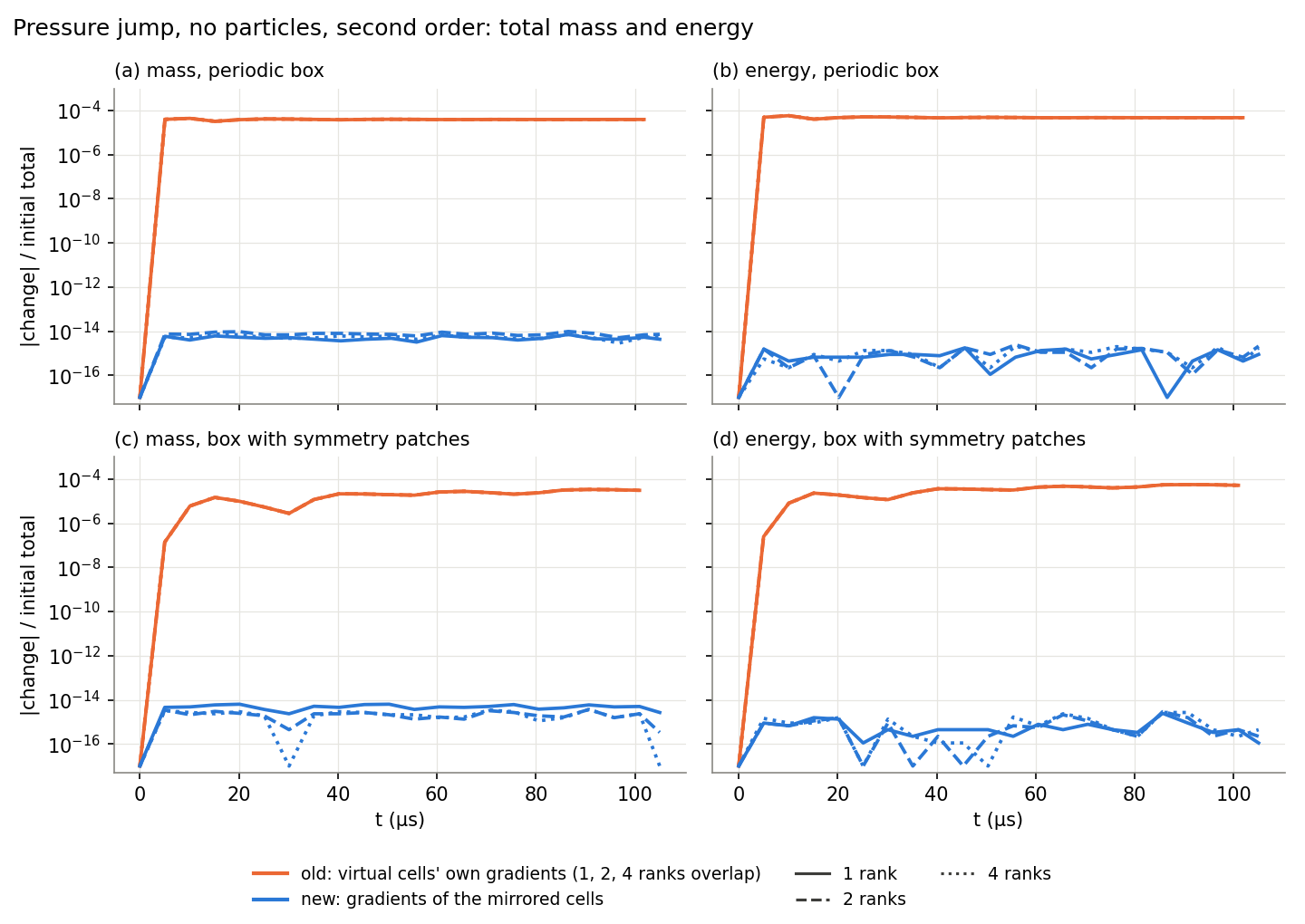
A pressure jump in a box without particles, at second order, with periodic patches (
box/gas-jump/periodic) and with symmetry patches on all six faces (box/gas-jump/symmetry). Before the fix, mass and energy drifted by 3–5e-5 within the first 10 µs, the same on 1, 2 and 4 ranks: the error came from the patches, not from MPI. Now both are conserved to 1e-14. -
Uninitialized reads (b10c5f1). The NSCBC patch
dvis set at initialization, and an out-of-bounds read ofdv(4)is fixed.
2D Runs
DIMENS 2 now runs the gas and the particles in 2D. ppiclF used to stop unless it was in
3D, and a 2D case had to be run as a thin 3D one. How to set a case up is in
Running a Simulation.
How It Works
DIMENS in the .inp sets ppiclf_ndim; there is no separate switch. The z direction
is inactive, not removed: PPICLF_JZ, PPICLF_JVZ and the rest keep their slots, so array
layouts and the restart format do not change. With ppiclf_ndim 2:
- Bins and ghosts: one bin in z and no ghosts in z.
- Interpolation, projection and neighbour search: the least-squares fit, the projection distance and the neighbour distance leave z out.
- Particle motion: z, v_z, ω_x and ω_y do not change.
- Particle walls: work as in 3D on the x and y patches.
Rocflu always has real 3D cells, so the mesh is one cell thick with two BC_VIRTUAL z
patches. The particles remain spheres in a slab of depth Δz, because the drag and heat
closures are for spheres. Δz is therefore the depth that sets the volume fraction, and
no separate characteristic width is needed.
Choosing the Thickness
For a target volume fraction φ, in-plane area A, particle diameter d and particle volume V_p:
| Quantity | Formula | Guidance |
|---|---|---|
| Number of particles | N = φ A Δz / V_p | |
| Area fraction in the plane | 1.5 φ Δz / d | Tested up to 0.30, so Δz ≤ 0.2 d/φ |
| Particles per cell | φ A_cell Δz / V_p | About 20 suggested: peak φ was 20% over target at 10 per cell, 7% at 38 (three runs only) |
At fixed φ, the thickness only sets N. On a Mach 1.27 shock over a bed (φ = 0.05, d = 100 µm, 1 mm cells, three beds at each Δz), mean particle velocity stayed within 0.4% and gas differences equalled the scatter between beds. Holding N fixed instead halved φ and moved the velocity by 4%.
Two Bugs Found on the Way
- Collisions and walls were silently off in 2D. Old branches in
ppiclf_user_subbinMap.fset no subbins in z, while the neighbour search and wall lookup still computed a z index. The 3D suite passed; only a 2D collision test caught it. - The thickness set the time step.
RFLU_TimeStepInviscidcounted virtual faces in the CFL sum: 403, 569 and 2227 steps at Δz = 10, 1 and 0.1 mm. They are now left out: 385 steps at all three, with gas fields equal to 4e-15.
How It Was Checked
- Regression suite: 21 cases under
2d/(Regression Tests) repeat the 3D coupling, interpolation, projection, collision, wall and gas-conservation tests in the plane, and check that nothing leaves the plane. - 3D results: dumps stayed byte-identical to the commit before the 2D work (502 files).
- Case validator: rejects a mesh more than one cell thick, virtual patches that are not
the z faces, particles off the mid-plane, nonzero v_z, and
PERIODICZ 1.
The Wedge against 3D
The first use is a 1° wedge: a Mach 41 shock into a thin bed of 40 µm particles, 20 µs, with AUSM+UP at second order and slip sides. The 2D case uses the first layer of the 3D grid's cells and the same volume fraction.
| Run | Ranks | Solver time | Steps | Bed width (mm) | Mean r (m) | Mean v_r (m/s) |
|---|---|---|---|---|---|---|
| 3D, 1 mm, 40,781 particles | 32 | 1659 s | 10011 | 42.3 | 0.34580 | 6188 |
| 2D, 100 µm, 4,078 particles, bed 1 | 32 | 139 s | 7406 | 38.7 | 0.34652 | 6259 |
| 2D, 100 µm, bed 2 | 32 | 147 s | 7406 | 40.3 | 0.34609 | 6210 |
| 2D, 125 µm, 5,098 particles | 16 | 148 s | 7406 | 38.7 | 0.34657 | 6261 |
Bed width is the 5th to 95th percentile of r at 20 µs. 2D is about 11 times faster, and the bulk of the gas overlays 3D.
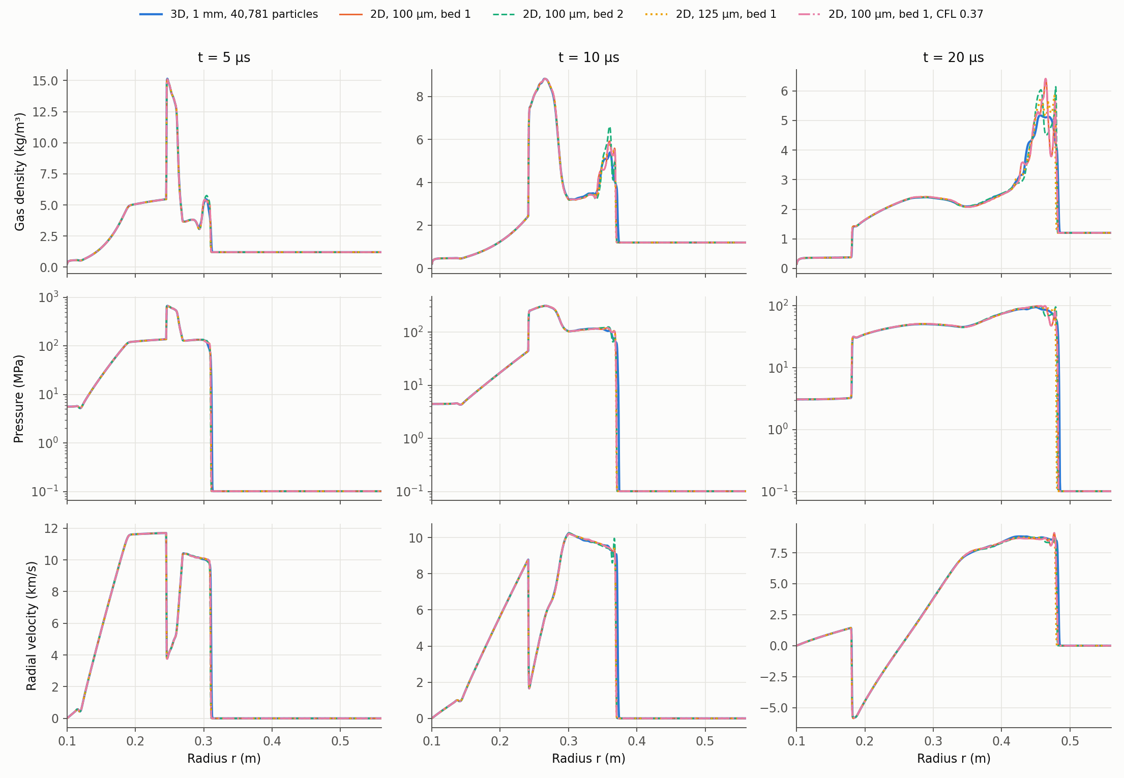
Three differences remain. The leading shock in 2D trails 3D by 1.3–1.8 mm at 5 µs, 3.0–3.9 mm at 10 µs and 2.1–4.3 mm at 20 µs. Behind the shock, 2D density and pressure oscillate and differ between beds; 3D is smoother, though it also averages five times more cells per radial bin. The 2D bed is 5–9% narrower with sharper pile-ups, against 1.7 mm of scatter between beds.
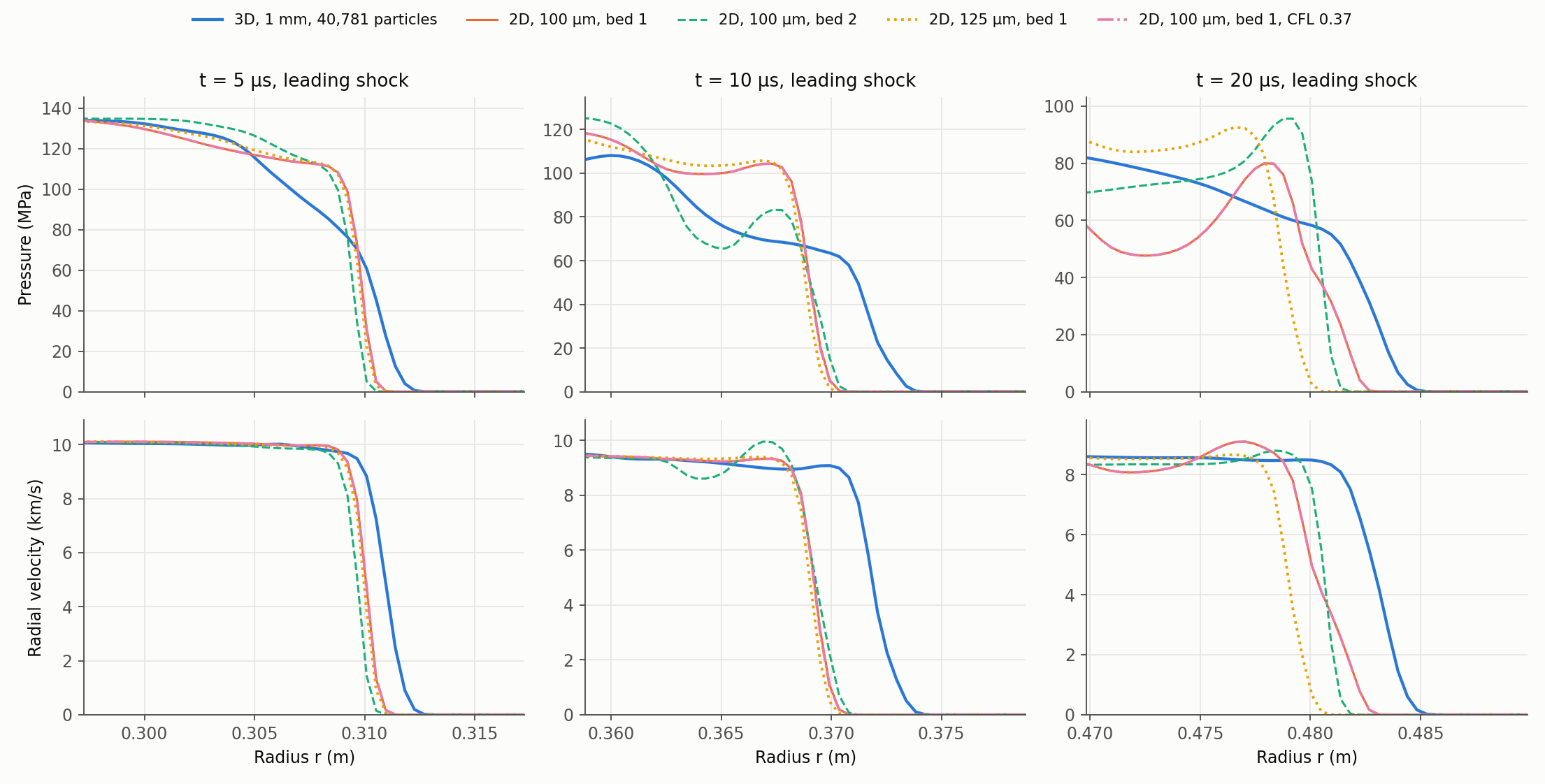
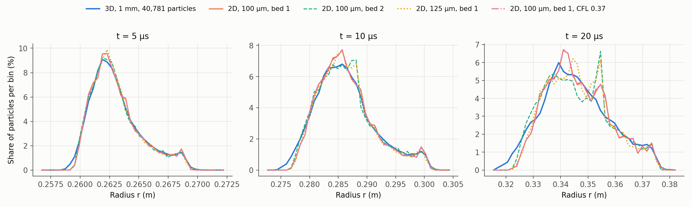
Matching 3D's time step (CFL 0.37, 9992 steps) leaves the shock difference unchanged, and it is still there with no particles. It comes from the gas numerics, described next.
Strong-Shock Numerics: Open Findings
These results are under validation. They describe the current behaviour of the gas solver at one very strong shock. The mechanism has not been measured, and no solver code was changed because of them. All runs are gas only.
The Test
The wedge's initial states (ρ 7.2076, u 11,833 m/s, p 2.0265e8 Pa into ρ 1.2048, p 101,325 Pa, γ 1.4) form a single shock at 14,207.9 m/s, with an exact solution. The wedge grid was remapped to a planar tube of 1499 × 24 cells (0.434 × 0.271 mm), 1 layer in 2D and 5 in 3D:
- Aligned: the shock is parallel to the cell faces.
- Sheared by 30°: side walls and flow stay along x, and the shock crosses the cells at an angle.
The flow should stay exactly 1D, so any transverse velocity is a numerical error.
Results
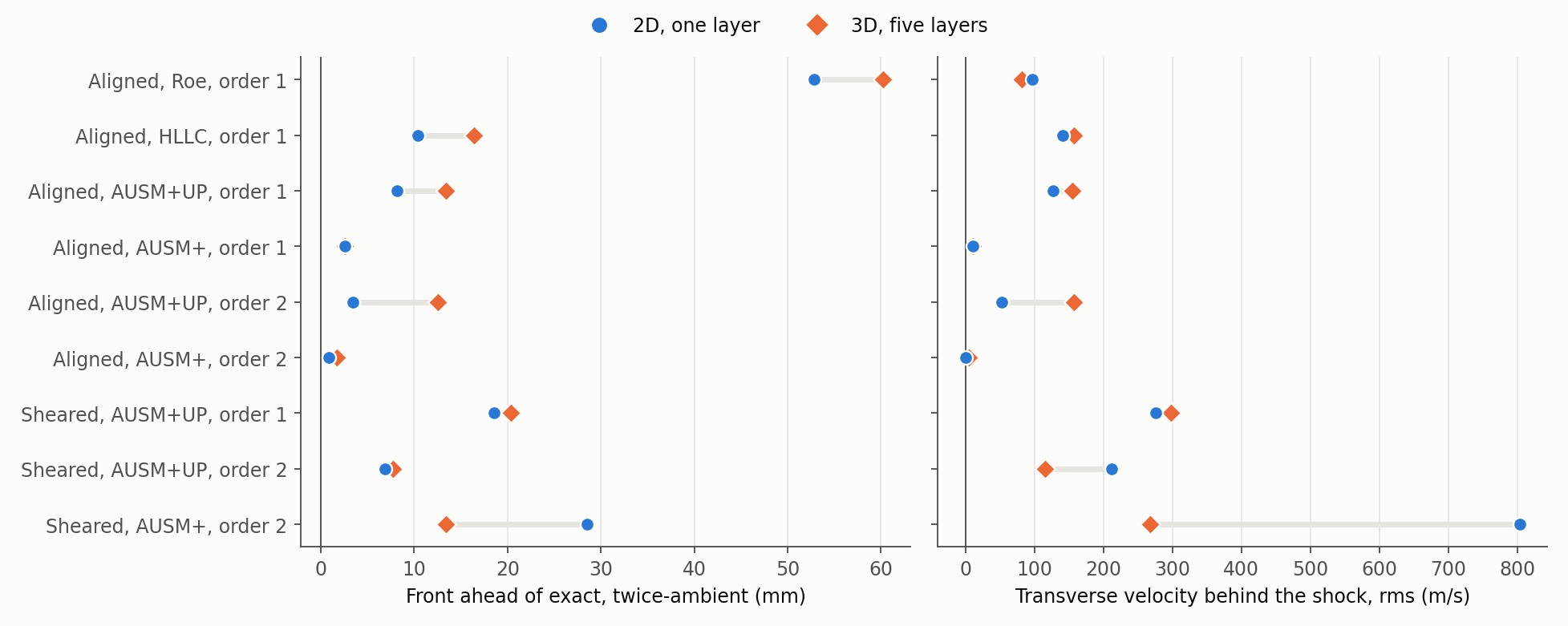
| Mesh | Scheme | ORDER |
Front error, twice ambient, 2D / 3D (mm) | Pressure error behind the shock, 2D / 3D (%) | v rms, 2D / 3D (m/s) |
|---|---|---|---|---|---|
| Aligned | Roe | 1 | +52.85 / +60.22 | -37.7 / -38.5 | 97 / 82 |
| Aligned | HLLC | 1 | +10.35 / +16.43 | -8.6 / -13.4 | 141 / 157 |
| Aligned | AUSM+UP | 1 | +8.19 / +13.39 | -5.7 / -7.8 | 127 / 155 |
| Aligned | AUSM+ | 1 | +2.55 / +2.55 | -0.17 / -0.16 | 10.6 / 10.6 |
| Aligned | AUSM+UP | 2 | +3.42 / +12.52 | -2.7 / -13.8 | 53 / 158 |
| Aligned | AUSM+ | 2 | +0.81 / +1.68 | 0.00 / +0.03 | 0 / 4.8 |
| Sheared | AUSM+UP | 1 | +18.59 / +20.33 | -8.0 / -7.3 | 276 / 298 |
| Sheared | AUSM+UP | 2 | +6.89 / +7.75 | -5.9 / -8.3 | 212 / 116 |
| Sheared | AUSM+ | 2 | +28.57 / +13.39 | -19.2 / -15.6 | 804 / 268 |
The front is the largest bin with mean pressure above twice ambient, at 20 µs; the exact shock is at x = 0.53216 m. Other scheme, order and mesh combinations have not been run.
On the wedge itself, the 2D grid was refined in plane:
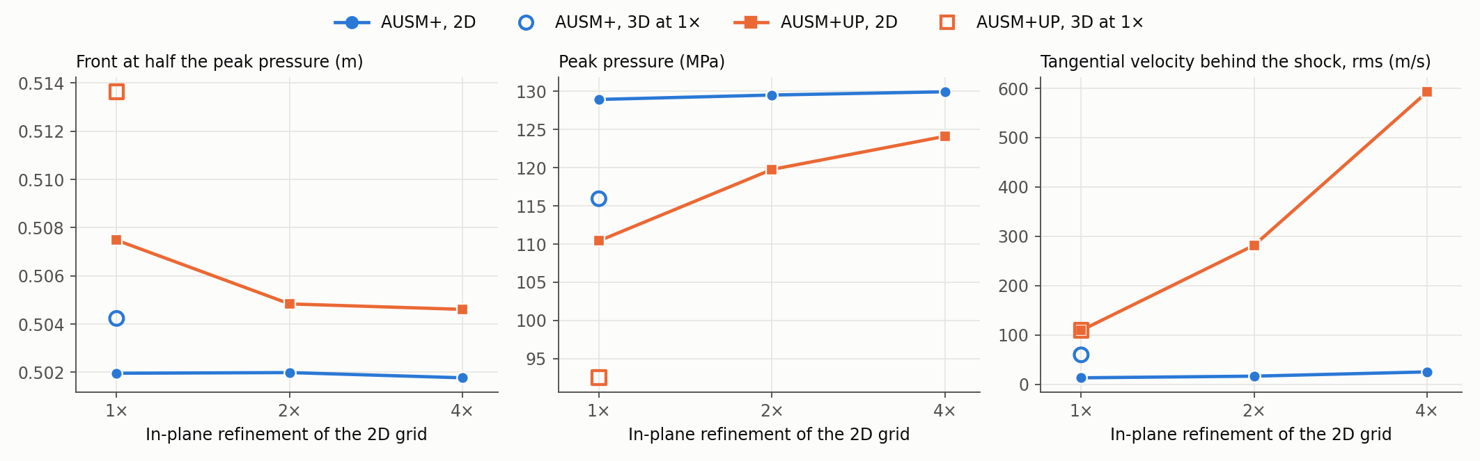
| Scheme | Grid | Front at half the peak pressure (m) | Peak pressure (MPa) | Tangential velocity rms (m/s) |
|---|---|---|---|---|
| AUSM+ | 2D 1×, 2×, 4× | 0.5020, 0.5020, 0.5018 | 128.9, 129.5, 130.0 | 13, 17, 25 |
| AUSM+ | 3D 1× | 0.5042 | 115.9 | 60 |
| AUSM+UP | 2D 1×, 2×, 4× | 0.5075, 0.5048, 0.5046 | 110.4, 119.8, 124.1 | 110, 282, 593 |
| AUSM+UP | 3D 1× | 0.5136 | 92.5 | 110 |
The wedge's tangential velocity is not zero even in a clean run, because the initial flow points along x rather than along r.
What Is Established
- Transverse velocity grows from zero behind this shock and the front runs ahead of exact, in 2D and 3D, at both orders. Reconstruction is not the root cause.
- It depends strongly on the flux scheme and the cell angle. AUSM+ is nearly exact on aligned cells and worse than AUSM+UP on sheared cells. Roe is the worst on aligned cells.
- 2D and 3D agree until z velocity grows, then split. This is timing only; cause is not shown.
- Which of 2D and 3D is closer to exact varies by case.
- On the wedge, refinement does not remove AUSM+UP's growth in tangential velocity.
What Is Not Established
- The mechanism. A carbuncle-type shock instability fits the symptoms but has not been tested directly.
- Whether AUSM+UP's behaviour comes from the published scheme or from this implementation.
- The wedge's true answer. AUSM+ gives about 0.502 m and is grid-converged, but this is one scheme, and the two still differ by 2.8 mm at 4×. No 3D run was refined.
- How far this reaches: only this Mach 41 state was tested, and only without particles.
Until this is settled, treat shock position at this strength as dependent on the scheme, and check it on the mesh in use. AUSM+ is not a general fix.
Gradients for Particle Forces
The particle models read gas gradients at each particle. Before, these were the gas
solver's own cell gradients (gradCell), which are smoothed by WENO and limited so that the
flux reconstruction stays stable. At a shock, that smoothing gave a particle 58% of the
pressure-gradient impulse. The particles now get their own least-squares gradients, without
smoothing, and receive the full impulse. The gas solver is unchanged.
What the Particles Receive
| Gradient | Used by | Computed when |
|---|---|---|
| ∇p | Pressure-gradient force, Parmar added mass, baroclinic term of the vorticity derivative | PGFORCE 1, AMFORCE 1 or COLLISIONS ≥ 2 |
| ∇(φρ) | Added mass, viscous unsteady, vorticity derivative | AMFORCE ≥ 1, VISCOUSUNSTEADY ≥ 1 or COLLISIONS ≥ 2 |
| ∇u, ∇v, ∇w | Vorticity and its derivative (torque, lift) | COLLISIONS ≥ 2 |
| ∇ρ_g | Added mass, viscous unsteady | AMFORCE ≥ 1, VISCOUSUNSTEADY ≥ 1 or GRADRHO_WRT 1 |
The first three go into piclGradCell, and ∇ρ_g into piclgradRhog. gradCell keeps
feeding the gas reconstruction as set by RECONST; changing it would change the gas
flow. A case with drag only computes none of these gradients. Before, ∇ρ_g was computed in
every stage. The conditions are in PICL_GradientNeeds (rocpicl/PICL_ModGradients.F90) and
match the fields ppiclf_user_Layout interpolates, so the two must be changed together.
Why Not the Gas Gradient
The test is a Riemann problem: 4.0 kg/m³ at 6.0e5 Pa against the pre-shock state of the
planar curtain (0.972 kg/m³, 82.7 kPa). It runs on 0.25 mm cells with HLLC and RECONST 2,
and is compared at t = 60 µs. The gradient is computed four ways on the same flow state:
least squares, and least squares with WENO, with the limiter, and with both (the old
gradient). The exact values are cell averages of the exact solution.
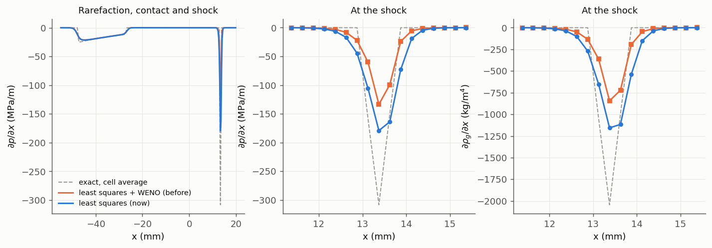
| At the shock | Least squares | Least squares + WENO (before) | Exact |
|---|---|---|---|
| ∫ ∂p/∂x dx across the shock, against Δp | 100% | 58% | 100% |
| ∫ ∂ρ_g/∂x dx across the shock, against Δρ | 100% | 58% | 100% |
| Peak ∂p/∂x (MPa/m) | −179 | −134 | (−308 as a cell average; the true front has no width) |
In the rarefaction the two differ by 0.1%. The limiter changed no cell, here or in the curtain below: it acts only where a face value would be ≤ 0, that is, near vacuum.
WENO-XYZ replaces each cell's gradient by a weighted mix of its neighbours' gradients, weighted towards the smallest. A shock is smeared over two or three cells, so the smallest gradient nearby is the one just outside it, and part of the jump is lost. That keeps the reconstruction stable. For a force it means the particle sees a smaller pressure jump than the gas has.
The same comparison on a copy of the planar curtain (1.8M cells, bed 0–2 mm, 8 cells across, φ_p up to 0.29, two-way coupling). Weighted by particle volume, |∇p| with WENO was 0.67 of least squares as the shock entered the bed (10 µs) and 0.77–0.83 afterwards. For |∇ρ_g| it was 0.68 and then 0.73–0.77. The differences are at the bed edges, where φ_p jumps:
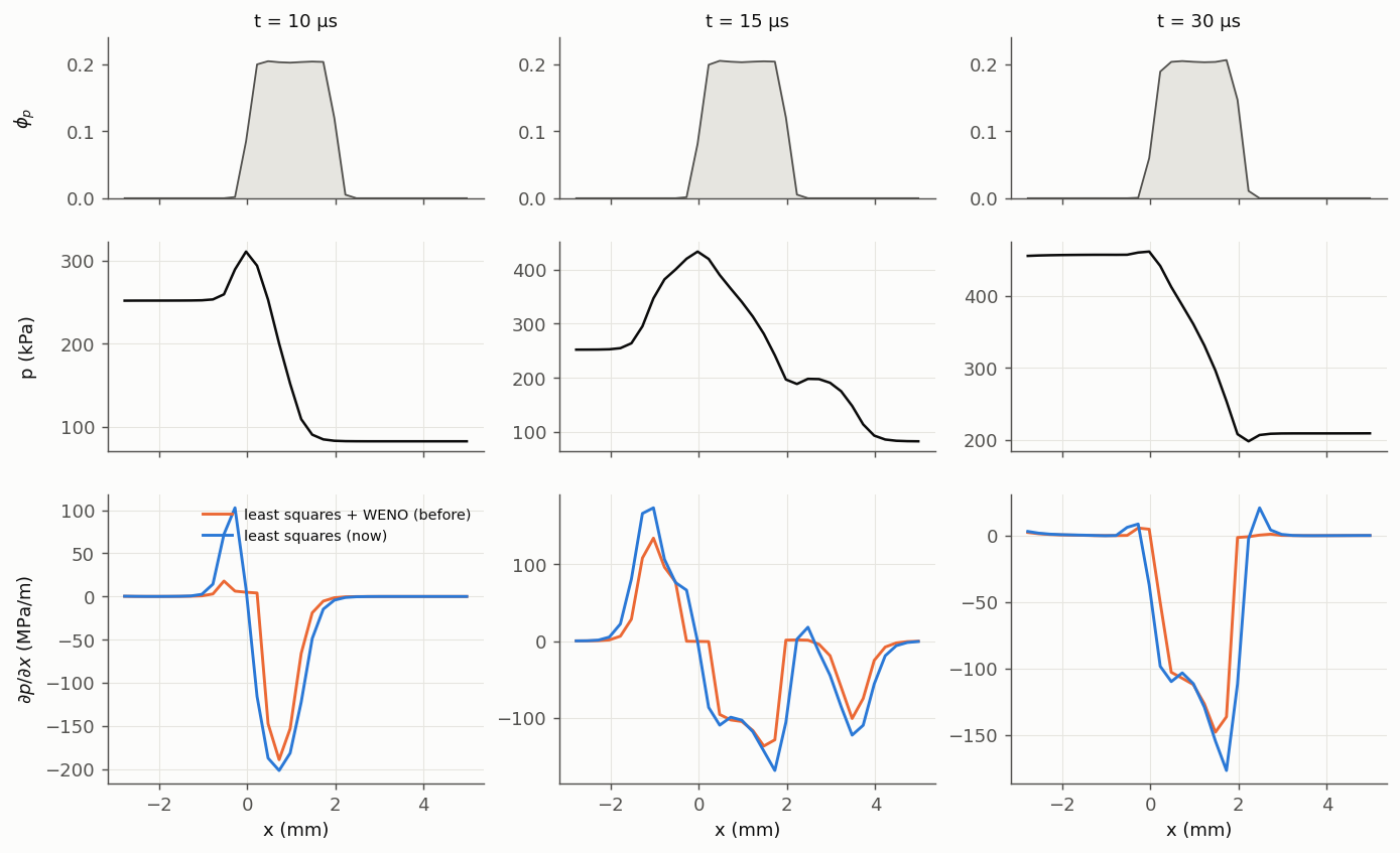
Effect on the Forces
Six particles are held fixed in the same tube, one-way, with PGFORCE 1 and AMFORCE 1.
The gas is the same in both runs, so only the gradients differ. For a fixed particle the
exact pressure-gradient impulse is V_p Δp / V_shock at the shock and V_p ∫ ∂p/∂x dt in the
rarefaction.
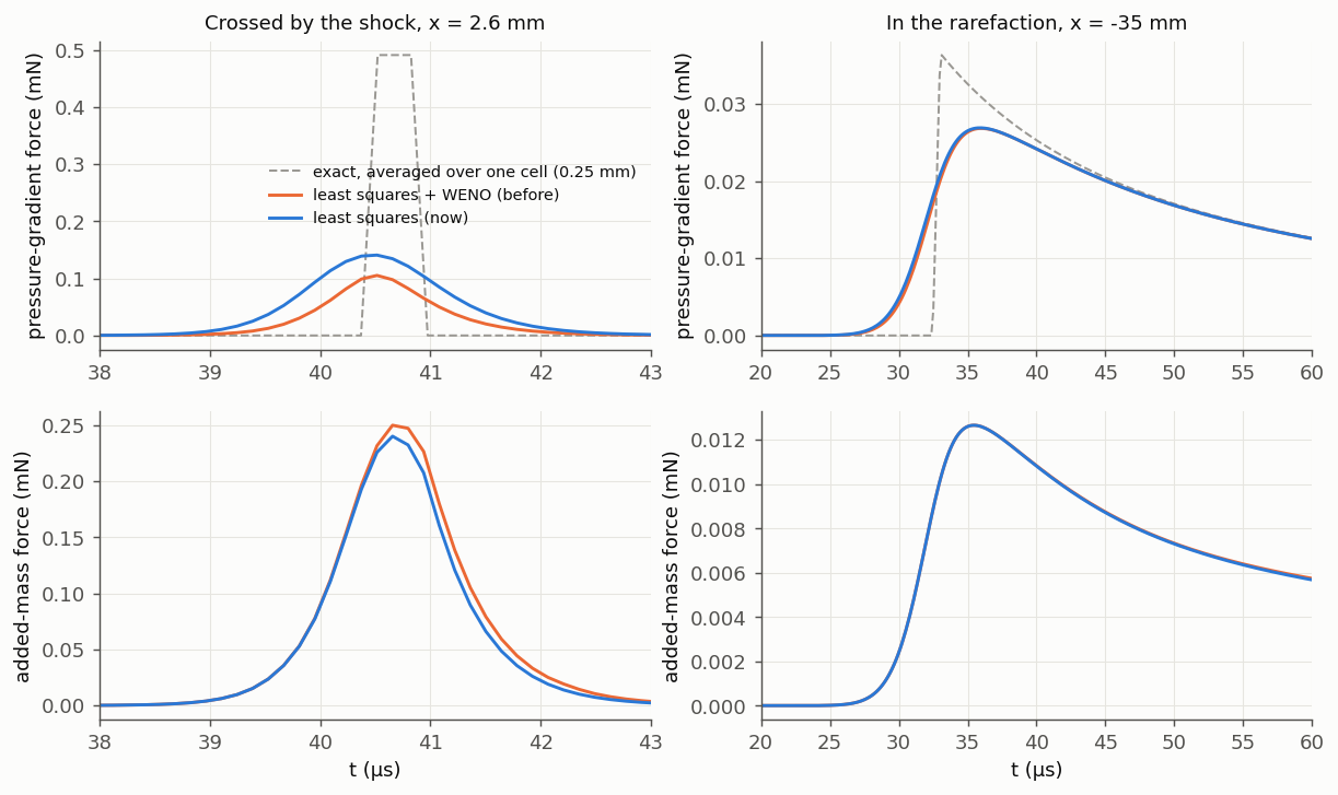
| Particles | Passed by | Pressure-gradient impulse: exact | Before | Now | Added-mass impulse: before | Now |
|---|---|---|---|---|---|---|
| x = −10.1, −4.9, 2.6, 7.4 mm | shock | 2.206e-10 N s | 1.282e-10 (58%) | 2.207e-10 (100%) | 3.43e-10 N s | 3.13e-10 (−9%) |
| x = −35 mm | rarefaction | 5.81e-10 | 5.70e-10 (98%) | 5.74e-10 (99%) | 2.60e-10 | 2.59e-10 |
The added-mass force uses ∇ρ_g through u·∇ρ_g. That term opposes the rest of the force, so it lowers the impulse by about 10% at the shock. There is no exact reference for the added mass yet.
Why a Quadratic Fit
A linear least-squares fit is exact for a linear field. It needs a stencil with neighbours on all sides. Some cells don't have one:
- Next to a wall, an inflow or an outflow: the neighbours are all on one side.
- Where two periodic directions meet: three neighbours are missing (see Still Open).
In those cells the fit turns curvature along the flow into a transverse gradient of order Δx ∂²p/∂x². At a shock that is large.
The fit used now adds the second derivatives that the stencil can resolve. It drops the ones
it cannot separate from the gradient, such as the curvature across a wall when there is one
cell layer. In a symmetric stencil it gives the same gradient as the linear fit. Its weights
are 1/|d|², as in Rocflu's linear fit, and are computed once per region. No wall constraints
(CRECONSTC) are applied to these gradients.
| Shock cells, transverse / streamwise gradient | Linear fit | Quadratic fit |
|---|---|---|
| Slip walls (8 × 8 cells of 1 mm), next to one wall | 0.30 | 2.2e-4 |
| Slip walls, wall corners | 0.21 | 1.4e-4 |
| Slip walls, away from the walls | 2.2e-4 | 2.2e-4 |
| Periodic (4 × 4 cells of 0.25 mm), corners | 0.061 | 7e-12 |
| Periodic, other cells | 3e-12 | 7e-12 |
What is left next to the walls is in the flow itself. Between the slip walls the pressure varies by 2.8 Pa across the 8 mm section without feedback and by 4.9 Pa with it, which is 1.6–2.7e-4 of ∂p/∂x times Δx. The streamwise gradient is the same in both fits to four digits everywhere. The tube, curtain and force results above were measured with the linear fit for that reason.
The Same Shock in MFC
MFC (master 7b16d32f) was run on the same problem and grid, with the numerics of its
2D_particle_curtain example (WENO5 mapped, HLLC, RK3). Its particles get
(q_R − q_L)/Δx from each cell's WENO face states. Its gas momentum source, the other half
of the two-way exchange, uses a central difference.
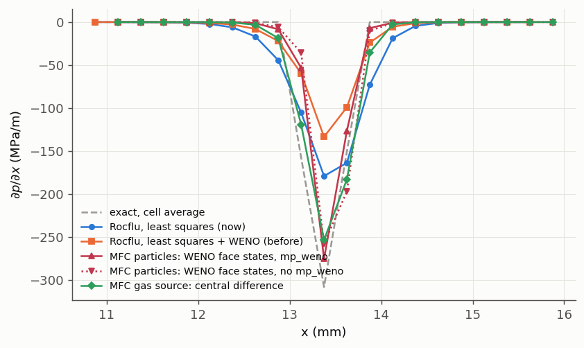
| Gradient | ∫ ∂p/∂x dx across the shock, against Δp |
|---|---|
| Rocflu, least squares (now) | 100% |
| Rocflu, least squares + WENO (before) | 58% |
MFC particles, WENO face states, mp_weno |
77% |
MFC particles, WENO face states, no mp_weno |
83% |
| MFC gas source, central difference | 100% |
MFC's shock is two to three cells wide, against four to five in Rocflu, so its peaks are higher. Its particle gradient also loses part of the jump. Because its gas source keeps the whole jump, the two halves of the two-way exchange do not match at a shock. This was read from the code and not measured.
How It Is Checked
shocktube/one-way/pg-impulse(new): the pressure-gradient force alone on two particles, which must gain the exact impulse within 2%. They are 0.9% and 1.4% low on its 1 mm cells. The old gradients gave 38% and 40% low.linear_grad_rhog(inbox/linear-interp): ∇ρ_g of a linear density is exact in every cell, walls included.- The Fortran fit agrees with an independent Python fit on the same stencils to 1.5e-12.
- Goldens changed with the gradients:
shocktube/two-way/pressure-gradient(particle speed +3.5%), the twoshocktube/slip-wallscases,shocktube/two-way/viscous-unsteady(+0.8%), andbox/quiescent-cloudon 2 and 4 ranks (round-off in gas at rest).
Limits
- No wall constraints. These gradients apply no wall constraints: next to a slip wall the wall-normal velocity has no wall value in the fit. Pressure and density never had one.
- No exact added-mass reference. The −10% in the added mass is measured but not checked against an exact value.
- Not measured on non-Cartesian grids. Interior cells of stretched or unstructured grids (the wedge) were not measured. There the quadratic fit differs from the linear one.
- ∇F is unchanged. The gradient of the projected feedback force, used in the torque, still uses least squares with WENO. It is a particle field, not a gas field.
Still Open
Gas numerics:
- Instability behind very strong shocks. See Strong-Shock Numerics.
- Missing virtual cells where two periodic directions meet. Cells there have 23 stencil
members instead of 26. The three cells across both periodic patches at once are never
built, because
RFLU_SYPE_AddVirtualCellshandles one patch at a time, and a later patch does not see the earlier one's virtual cells. A linear field is still fitted exactly. A curved one gets a false transverse gradient, 6% of ∂p/∂x at a shock, in the gas reconstruction (partly hidden by WENO). The particle gradients are not affected (see Why a Quadratic Fit).
Collision model:
-
The normal force turns attractive at the end of a contact. The normal force is −k δ − η v_n. While the particles separate, v_n changes sign, and near the end of the contact the dashpot term exceeds the spring term. The animation of the binary collisions shows a pull of 1–2% of the rebound speed. The usual fix allows only repulsive normal forces (clip at 0, as in LIGGGHTS). Clipping removes some damping, so the actual e comes out above EREST unless η is recalibrated (linear spring–dashpot, Schwager & Pöschel 2007):
EREST e with clipping 0.5 0.550 0.7 0.718 0.9 0.902 The friction and rolling torques use |F_n|, so they also act during the attractive phase. The code keeps the unclipped force for now.
-
min(k₁, k₂). ppiclF takes the softer of the linear stiffness k₁ and the Hertz stiffness k₂. In the Hertz branch e depends on the impact speed (0.725 for an equal pair at 2 m/s).
-
Material constants. E = 1 GPa and ν = 0.35 are fixed in the code for every particle and wall. Aluminium is about 70 GPa.
-
Resolution. KSP·dt sets the contact time, so fast impacts penetrate by v·KSP·dt/π (see above). A time-step limit from the particle speeds would bound it.
Known limitations:
- Walls that only the particles see (a screen or an obstacle that is not in the fluid
mesh) are not supported since
filein.vtkwas removed. - In the closed box of
box/wallsthe gas seen by the particles differs between 1 and 2 ranks by about 0.2% of a 4e-4 m/s flow (driven by φ withFEEDBACK 0). The particles agree; the gas difference is not explained yet. - Ghost particles are created and sent in every RK stage, even when nothing uses them.
- The subbin start index in
ppiclf_user_SetYdotis declared for every subbin even when no neighbour search runs. Subbins areNEIGHBORWIDTH(at least 4 dp) wide, so very small particles withNEIGHBORWIDTH 0give a huge count (about 40 GB of address space for 1 µm tracers in a 4 cm tube; it is never touched). - The quasi-steady fluctuation mean (
QSFLUCT) only sees neighbours withinNEIGHBORWIDTH, not the filter width it is meant to average over. - Feedback lags one RK stage, because particles are projected before
ppiclf_user_SetYdot. It conserves, but the coupling is first order in time. - Restart from a PICL dump is not verified: the files hold ρ/(1−φ), and the particle VTU files that restarts read are single precision.
FEEDBACK 0(one-way) still changes the gas through φ in the pressure.- PICL supports only one region per MPI rank, and there is no check for this.
Reproducing the Figures
The particle-gradient figures are drawn by figures/src/particle_gradients/plot.py from
data.json next to it. extract.py wrote that file from the runs behind
Gradients for Particle Forces. Those runs used a
diagnostic build of e7f0952
(each gradient variant written on the same flow state, a particle force log) and MFC
master 7b16d32f with its face states written out. They are not part of the repository.
Each figure compares the commit before a fix with the commit after it. The run and plot
scripts (sweeps.py, make_plots.py, qs_driver.F) are kept locally under the
git-ignored tests/_work/plots/. They need a built tree of each old commit
(aa3c0b6, 6d00ca4, 1a954d7, eb59a6c) as well as the current one.
The collision figures use the same folder: animate_collisions.py animates a run of
box/binary-collisions written every 0.1 µs; walls.py sets up and runs the wall probe
(WALLS=vtk or WALLS=patch, SHOTS= a subset) with any built tree, and
animate_walls.py and wall_summary.py draw the animation and the summary figure from
the old (3afd23a) and new (2ff0cd8) probe runs. shock_interp.py (planar shock),
static_interp.py (tracers across the cells at one instant), periodic_ghosts.py
(collisions through periodic boundaries) and sheet.py (particle
sheet, run, runpoly, plot2, animate; its runs went to Slurm on hpg-dev, 8 ranks
each) run and plot the interpolation comparisons in shock-driven flow, with aa3c0b6 as
the old interpolation.
For the MPI and boundary figures, run_all.sh runs mpi_periodic.py (the gas-jump box
with periodic or symmetry patches, and the quiescent cloud) on 1, 2 and 4 ranks with built
trees of 47b0940 (before
11dc640),
8885909 (before
e3ed370) and the current code,
each with its own test harness; plot_mpi_periodic.py draws both figures from the saved
totals.
The 2D and strong-shock figures are the exception: their scripts and compact results are
in the repository under docs/figures/src/strong_shock/. plot_results.py redraws both
strong-shock figures from results.json. remap.py and refine.py make the grids from the
wedge grid, exact.py gives the exact solution, compare.py, front_rows.py and
ref_compare.py read the runs, and make_wedge_2d.py, profiles.py and plot_wedge.py
build the 2D wedge case and draw its figures. Their paths point at the original run
directories, so edit those to rerun.
The interpolation comparison: tests/_work/interp_model/interp_compare.py (Python, no
build needed) computes all four methods and draws the figure.
The heat transfer figures: tests/_work/plots/heat_transfer/ holds ext5.py and
ext8.py (read the PR-DNS points from Sun et al. 2015 Figs. 5 and 8, needs PyMuPDF),
ref.py (the published formulas), plot_ht.py and plot_theta.py (the figures and the
error tables), htdrive.f (calls the compiled models; linked against a built tree's
libppiclF.a) and htbox.py (the periodic box runs, given a built tree).